Solving XOR with a Perceptron
Solving the XOR problem using a simplel neural network
Objective
Solve the XOR problem using a simple neural network with backpropagation in Python.
Overview
We will first work through a simpler problem. Then we will use those tools for the XOR problem.
By the end you should be able to answer the following questions in addition to solving the XOR problem.
- What is the XOR problem?
- What is a neural network?
- What is forward propagation
- What is backpropagation?
- What is a learning rate?
Intro
In The Matrix Neo is plugged into a machine and downloads martial arts. If only life were this easy. Elon Musk’s NeuralLink is trying but hasn’t advanced that much…yet…we can still imagine how this could work.
 Quotes from my students on why they are taking physics.
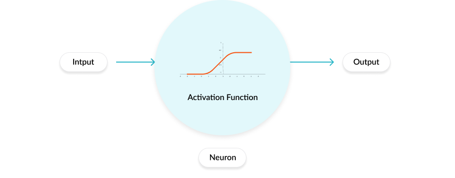
The brain is comprised of millions of neurons. A neuron either fires or doesn’t fire. When it comes to fighting our brain takes input from our environment, sends it to the neurons, and the result of all those neurons firing or not firing generates an action. On the single neuron level it looks something like this.
 Quotes from my students on why they are taking physics.
Notice not all input is useful and some is more useful than others. So we weigh each input to determine the proper action. We figure out the weights by making mistakes. We block when we should have kicked. We kick when we should have blocked.
When it comes to human training we general stick to the 10-Thousand-Hour rule. In other words, it takes 10k hours or 10k reps of doing something to figure out how to properly weight the inputs.
 Quotes from my students on why they are taking physics.
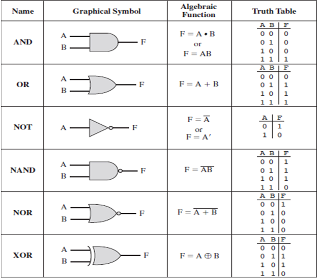
Unforuntately we, as humans, don’t always have the time to invest in mastery over a niche problem. So we teach machines how to learn because they can do it much faster than us. And: the basic building block of digital circuits are called logic gates. There are seven basic gates which are shown below.
 Quotes from my students on why they are taking physics.
With two inputs we can build the OR logic gate.
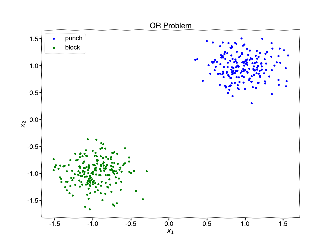
The OR Problem
Let’s analogize Neo fighting problem and translate it into Python. Given two inputs, {\(x_1:\text{hand moving towards Neo},x_2:\text{hand moving towards sky}\)}, should Neo block or punch?
# generating random dataset
import matplotlib.pyplot as plt

from sklearn.datasets import make_blobs
from sklearn.model_selection import train_test_split
from sklearn.preprocessing import StandardScaler

plt.xkcd()

# generate data
#centers = [[1, 1], [-1, -1], [1, -1],[-1, 1]]
centers = [[1, 1], [-1, -1]]
X, Y = make_blobs(n_samples=400, centers=centers, cluster_std=0.25,random_state=0)
X = StandardScaler().fit_transform(X)

# reset labels
#Y = np.array([0 if (YY == 0) else 1 for YY in Y ])

# plot data
plt.figure(figsize=(16,12))
plt.rcParams.update({'font.size': 22,'font.family': ['Helvetica']})

colors = ['blue','green'] # colors for plotting
for i in range(0,2): # loop over {'block','punch'}
    flag = (Y==i)
    plt.scatter(X[flag,0], X[flag,1], c=colors[i],label=str(i))
plt.xlabel('$x_1$')
plt.ylabel('$x_2$')
plt.legend(['punch','block'])
plt.title('OR Problem')
plt.savefig('figure1.png')
plt.show()
 Quotes from my students on why they are taking physics.
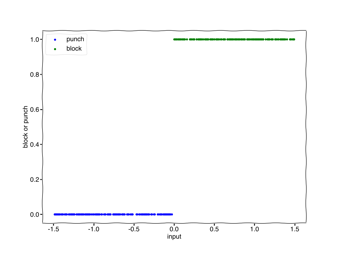
Given the inputs we need to decide on block or kick. We can visualize the output as zero for block and one for punch, {\(block:0, punch:1\)}.
import numpy as np

plt.figure(figsize=(16,12))
plt.rcParams.update({'font.size': 22,'font.family': ['Helvetica']})

colors = ['blue','green'] # colors for plotting
for i in range(0,2):
    if i ==0:
        n = len(Y[(Y==i)])
        xx = np.random.uniform(-1.5, 0, n)
    else:
        n = len(Y[(Y==i)])
        xx = np.random.uniform(0, 1.5, n)
    plt.scatter(xx, Y[(Y==i)], c=colors[i],label=str(i))

plt.legend(['punch','block'])
plt.xlabel('input')
plt.ylabel('block or punch')
plt.savefig('figure2.png')
plt.show()
 Quotes from my students on why they are taking physics.
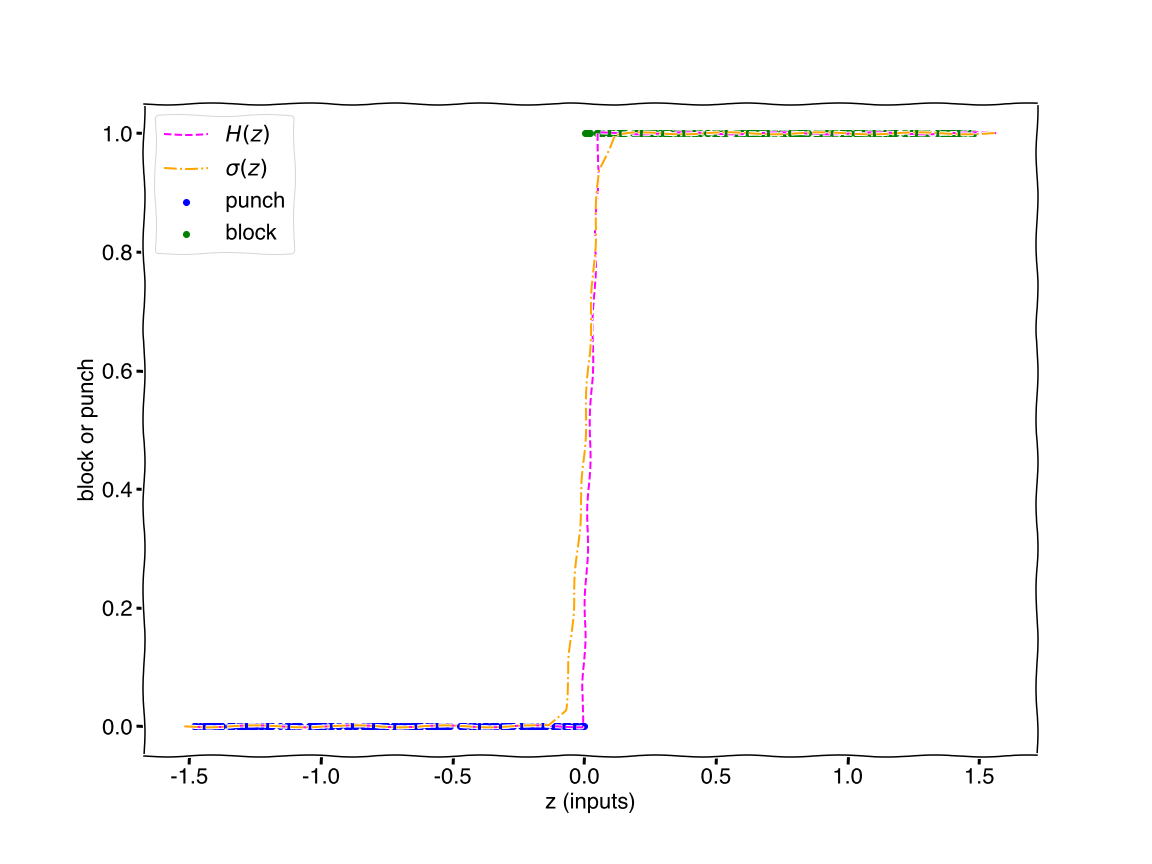
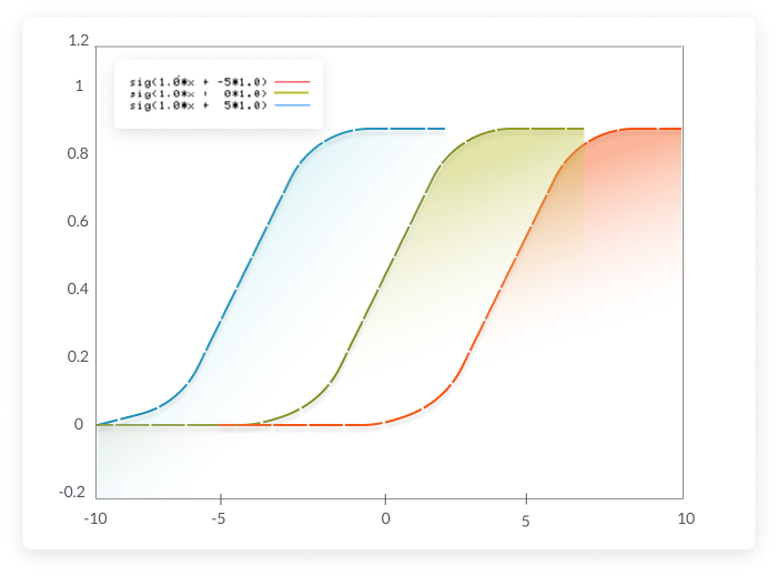
Notice our problem is a classification task and we just need a function that can map our inputs to a binary output. Two functions which are perfect for this, (1) the step function (aka Heaviside step function) and (2) the sigmoid function. They are plotted below.
import numpy as np
from scipy.special import expit

def step_func(z):
    return np.where(z<0,0,1)

def sigmoid(z):
    return 1/(1+np.exp(-z*50))

plt.figure(figsize=(16,12))
plt.rcParams.update({'font.size': 22,'font.family': ['Helvetica']})

z = np.linspace(min(X[:,0]),max(X[:,0]),50)
colors = ['blue','green'] # colors for plotting

for i in range(0,2):
    if i ==0:
        n = len(Y[(Y==i)])
        xx = np.random.uniform(-1.5, 0, n)
    else:
        n = len(Y[(Y==i)])
        xx = np.random.uniform(0, 1.5, n)
    plt.scatter(xx, Y[(Y==i)], c=colors[i],label=str(i))

plt.plot(z, step_func(z),'--',color='magenta')
plt.plot(z, sigmoid(z),'-.',color='orange',markersize=8)
plt.legend(['$H(z)$','$\sigma(z)$','punch','block'])
plt.xlabel('z (inputs)')
plt.ylabel('block or punch')
plt.savefig('figure3.png')
plt.show()
 Quotes from my students on why they are taking physics.
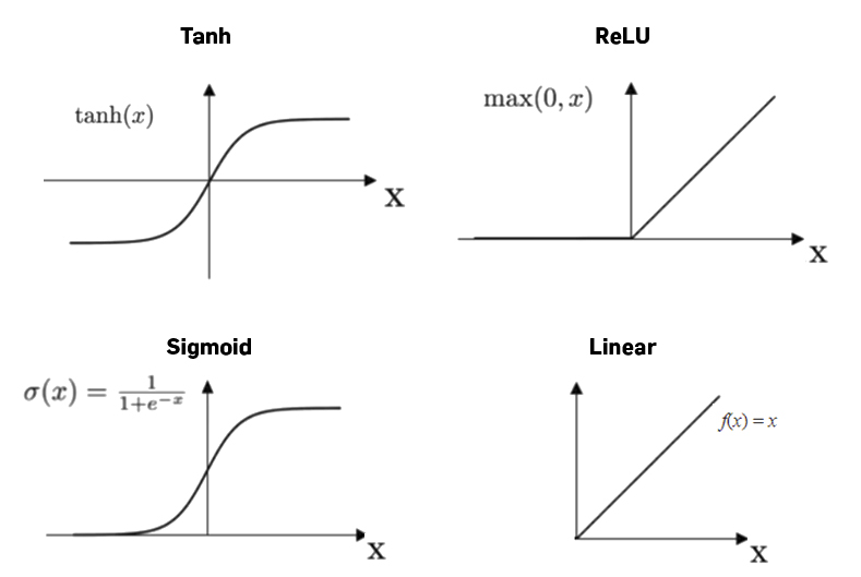
The sigmoid function is the standard when starting with “neural networks” as they are called. Although other “activation” functions are typically used in production.
Now that we have we an output function we need a way to feed this function our weighted inputs. The simplest method is a linear combination. Think of the classic equation \[y=mx+b\]
and let \(y\rightarrow z\) and \(m\rightarrow w\), so we have \[z=wx+b,\]
where and \(b\) is called the “bias”. With two inputs, our equation becomes \(z=w_1x_1+w_2x_2+b\)
If we shift our thinking to linear algebra we can think of our parameters \(w\) and \(x\) as vectors and rewrite our function. \[z=\hat{w}^T\hat{x}+b\]
where \(\hat{w}^T=(w_1,w_2)\) and \(\hat{x}=\left( \begin{array}{c} x_1\\ x_2\\ \end{array}\right)\). Therefore, to map our inputs to a binary output we use the sigmoid function with a linear combination of our weighted inputs and a bias. \[\begin{aligned} \sigma(z)&=\frac{1}{1+e^{-(\hat{w}^T\hat{x}+b)}} \\ &=\frac{1}{1+e^{-(w_1x_1+w_2x_2+b)}} \\ \end{aligned}\]
Let’s test this sigmoid function with some random weights for a randomly chosen set of inputs.
def sigmoid(z):
    return 1/(1+np.exp(-z))

weights = np.random.uniform(-1,1,size=2)
bias = np.random.uniform(-1,1,size=1)
print("\nWeights: ", weights)
print("\nBias: ", bias,"\n")

for _ in range(10):
    choice = np.random.randint(len(Y), size=1)
    x = X[choice].T
    z = np.dot(weights,x)+bias
    print("~~~ Iteration ~~~")
    print("Sigmoid Output (Prediction): ", 1 if sigmoid(z)[0] > 0.5 else 0)
    print("Label Output (Actual): ",Y[choice][0])
Weights:  [-0.14392506  0.19853951]

Bias:  [0.69993978]

~~~ Iteration ~~~
Sigmoid Output (Prediction):  1
Label Output (Actual):  1
~~~ Iteration ~~~
Sigmoid Output (Prediction):  1
Label Output (Actual):  1
~~~ Iteration ~~~
Sigmoid Output (Prediction):  1
Label Output (Actual):  0
~~~ Iteration ~~~
Sigmoid Output (Prediction):  1
Label Output (Actual):  1
~~~ Iteration ~~~
Sigmoid Output (Prediction):  1
Label Output (Actual):  0
~~~ Iteration ~~~
Sigmoid Output (Prediction):  1
Label Output (Actual):  1
~~~ Iteration ~~~
Sigmoid Output (Prediction):  1
Label Output (Actual):  0
~~~ Iteration ~~~
Sigmoid Output (Prediction):  1
Label Output (Actual):  0
~~~ Iteration ~~~
Sigmoid Output (Prediction):  1
Label Output (Actual):  1
~~~ Iteration ~~~
Sigmoid Output (Prediction):  1
Label Output (Actual):  0
We have a few correct in there. Let’s interate over the entire set to calculate the accuracy.
counts = 0
for k in range(len(Y)):
    x = X[k].T
    z = np.dot(weights,x)+bias
    guess = 1 if sigmoid(z)[0] > 0.5 else 0
    answer = Y[k]
    if guess == answer:
        counts += 1
print("Accuracy over entire dataset = {}%".format(100*counts/len(Y)))
Accuracy over entire dataset = 50.0%
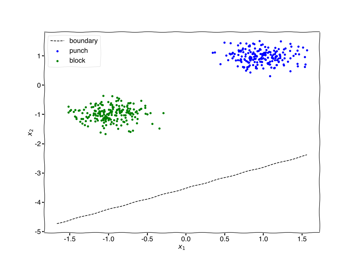
With random weights without 10k training reps we have 50% accuracy. For reference, let’s plot the decision boundary generated from the weights and bias.
# drawing decision line
x_ = np.linspace(X.min(),X.max(),100)
y_ = -(weights[0]*x_ + bias)/weights[1] # equation equivalent to y = m*x + b

plt.figure(figsize=(16,12))
plt.rcParams.update({'font.size': 22,'font.family': ['Helvetica']})
colors = ['blue','green'] # colors for plotting
for i in range(0,2): # loop over {'block','punch'}
    flag = (Y==i)
    plt.scatter(X[flag,0], X[flag,1], c=colors[i])
plt.plot(x_, y_, 'k--')
plt.xlabel('$x_1$')
plt.ylabel('$x_2$')
plt.legend(['boundary','punch','block'])
plt.savefig('figure4.png')
plt.show()
 Quotes from my students on why they are taking physics.
With the decision boundary so low why does it make sense that the accuracy is 50%? Answer
``` Assume our classes are balanced (50% of the data is class 0 and 50% is class 1). If we classify everything as one of the classes then we are guaranteed to be 50% correct. ```
How does the bias affect the sigmoid function? Answer
 ``` The bias shifts the sigmoid left and right. ```
Let’s make a 10k random weights and bias and retest the accuracy.
accuracy = []

for _ in range(10000):
    weights = np.random.uniform(-1,1,size=2)
    bias = np.random.uniform(-1,1,size=1)

    counts = 0
    for k in range(len(Y)):
        x = X[k].T
        z = np.dot(weights,x)+bias
        guess = 1 if sigmoid(z)[0] > 0.5 else 0
        answer = Y[k]
        if guess == answer:
            counts += 1
    accuracy.append(100*counts/len(Y))

plt.figure(figsize=(16,12))
plt.rcParams.update({'font.size': 22,'font.family': ['Helvetica']})
plt.hist(accuracy,bins=25)
plt.xlabel('accuracy (%)')
plt.ylabel('counts')
plt.title
plt.savefig('figure5.png')
plt.show()
 Quotes from my students on why they are taking physics.
Why three distinct peaks? Answer
``` Because of the decision boundary. Think of how the boundary should be made so have 50% accuracy. Any line where all the points are above or below the line. Now consider the large range of decision boundaries which have negative slope dividing the two groups. The tricky peak is the large peak for 0% accuracy. These would be the positive sloped decision boundaries which split the groups. ```
So the trick is to train the weights, and the way to train the weights is to adjust them based on their error. This concept of adjusting the weights after prediction is called back propagation while the concept of initializing weights and sending the inputs into the network to generate a prediction is called forward propagation.
Let’s use a random initialization of weights and bias and train them by adjusting the weights and bias by a fraction of the prediction error. Let’s also cleanup the code a bit and save a portion of the data to test improvement.
 Quotes from my students on why they are taking physics.
Perceptron
import numpy as np
import matplotlib.pyplot as plt


class Perceptron():

    def __init__(self):
        np.random.seed(1) # for consistency
        self.weights = np.random.uniform(-1,1,size=2).reshape(-1,1)
        self.bias = np.random.uniform(-1,1,size=1)

    def sigmoid(self, z):
        return 1/(1+np.exp(-z))

    def forward(self, X):
        predictions = self.sigmoid(np.dot(X, self.weights) + self.bias)
        return [1 if prediction > 0.5 else 0 for prediction in predictions]

    def backward(self, X, labels, prediction, alpha=0.1, ):
        # adjust weights and bias
        self.weights += alpha * np.dot(X.T, (labels - prediction)) # adjust the weights by a fraction of the absolute error
        self.bias += alpha * np.sum(labels - prediction) # adjust the bias by a fraction of the absolute error

    def train(self, X, labels, alpha=0.1, epochs=3):
        errors = []
        for t in range(epochs):
            # forward and backward propagation
            prediction = self.sigmoid(np.dot(X, self.weights) + self.bias).reshape(-1,1)
            self.backward(X,labels,prediction, alpha=0.1,) # adjust weights and bias

            # calculate error "loss" (MSE)
            loss = np.square(np.subtract(labels,prediction)).mean()
            errors.append(loss)
            print(f"epoch {t}/{epochs} loss: {loss}")

        # plot results
        plt.figure(figsize=(16,12))
        plt.rcParams.update({'font.size': 22,'font.family': ['Helvetica']})
        plt.plot(errors)
        plt.xlabel('epoch')
        plt.ylabel('loss (MSE)')
        plt.savefig('figure6.png')
        plt.show()
# generating random dataset
import matplotlib.pyplot as plt

from sklearn.datasets import make_blobs
from sklearn.model_selection import train_test_split
from sklearn.preprocessing import StandardScaler

plt.xkcd()

# generate data
centers = [[1, 1], [-1, -1]]
X, Y = make_blobs(n_samples=400, centers=centers, cluster_std=0.25,random_state=0)
X = StandardScaler().fit_transform(X)
x_train, x_test, y_train, y_test = train_test_split(X, Y, random_state=1) # split data


# training the model
model = Perceptron()
model.train(x_train,y_train.reshape(y_train.shape[0],1))
print(f'weights={model.weights} bias={model.bias}')
epoch 0/3 loss: 0.35352423104984243
epoch 1/3 loss: 1.6170039272565628e-14
epoch 2/3 loss: 1.6170022596452844e-14
 Quotes from my students on why they are taking physics.
weights=[[-16.3588014 ]
 [-15.74047103]] bias=[5.6024848]
After two training cycles, called epochs, the error has decreased to zero. The accuracy on the test set is given below.
counts = 0
for k in range(len(y_test)):
    x = x_test[k].T
    z = np.dot(model.weights.T,x)+model.bias
    guess = 1 if sigmoid(z)[0] > 0.5 else 0
    answer = y_test[k]
    if guess == answer:
        counts += 1
print("Accuracy over entire dataset = {}%".format(100*counts/len(y_test)))
Accuracy over entire dataset = 100.0%
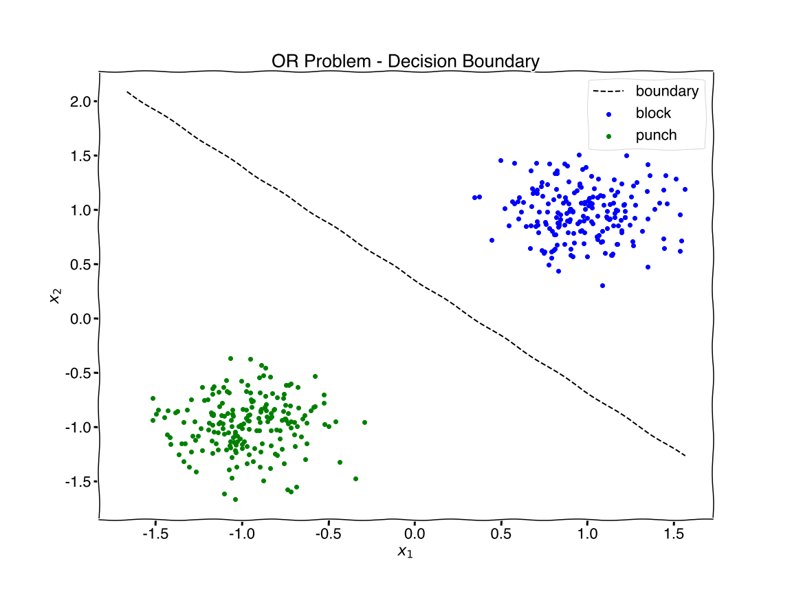
Now that we have trained our model let’s replot the decision boundary.
# drawing decision line
x_ = np.linspace(X.min(),X.max(),100)
y_ = -(model.weights[0]*x_ + model.bias)/model.weights[1]

plt.figure(figsize=(16,12))
plt.rcParams.update({'font.size': 22,'font.family': ['Helvetica']})

colors = ['blue','green'] # colors for plotting
for i in range(0,2): # loop over {'block','punch'}
    flag = (Y==i)
    plt.scatter(X[flag,0], X[flag,1], c=colors[i],label=str(i))

plt.plot(x_, y_, 'k--')
plt.xlabel('$x_1$')
plt.ylabel('$x_2$')
plt.title('OR Problem - Decision Boundary')
plt.legend(['boundary','block','punch'])
plt.savefig('figure7.png')
plt.show()
 Quotes from my students on why they are taking physics.
Review
We have just successfully simplified and analogized Neo’s block-punch dilemma as a classification problem using a simple model of a neural network. This simple neural network model is often called a “perceptron”. It works well for linearly seperable classification problems, such as this “OR” problem.
Everything dealing with neural networks beyond this is either to solve the problem more effiiently (ie. compute resources, time), more effectively (ie. higher accuracy, better generalizability), more complex problem (ie. more features, more complex decision boundary). For example, to better update our weights and bias we call “alpha” the learning rate and we can fine tune it or even make it adjustable.
A more complex problem is the “XOR” problem. Let’s explore the OR and XOR problem together using Tensorflow’s Playground
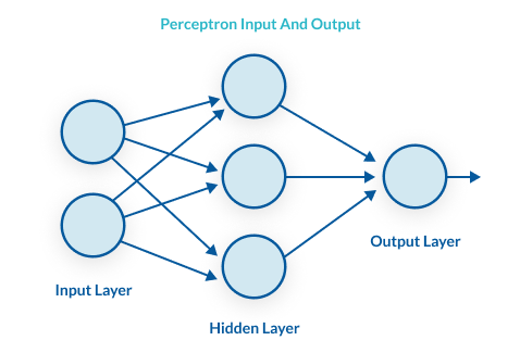
Multilayer Perceptron
The Tensorflow playground has shown us that we need one hidden layer with four neurons. The code we wrote only has no hidden layers. Therefore, we must modify our code to handle forward and backward propagation with multiple layers
Quotes from my students on why they are taking physics.
Generalized Forward Propagation
Recall that forward propagation is the process where we initialize weights and bias then send our input through the network to make a prediction.
For a larger, more complex network we need a generalized method of forward propagation. Since we now understand how to do forward propagation with a single neuron, which was our output neuron, we simply replicate the process for every other neuron. The main difference is the “input”.
Our inputs were \(x_1\) and \(x_2\), which we taken into the neuron to generate an output. Imagine another layer after this output, just as we will need to solve the XOR problem.
What is the input for this hidden layer? Answer
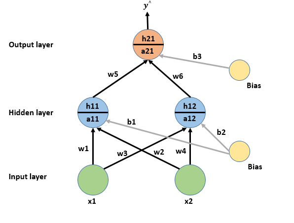{:.lead data-width="800" data-height="100"} Quotes from my students on why they are taking physics. {:.figure} ``` The new input is the output from the previous layer, which is the sigmoid activation output. The process can be written as follows. 1. Multiply each input by the first-layer weights {w1,w2, ...} and add a bias b1 2. Applying the activation function 3. Use output from activation function as input for next layer 4. Repeat steps 1-3 until last layer reached 5. Last output is the prediction of the neural network. ```
How many bias parameters should we expect for a given network? Answer
``` One per neuron to shift each neuron output ```
PSEUDO-ISH CODE
Example 1
# FOR A SINGLE TRAINING EXAMPLE
x = np.array([-1,-1]) # training example
layers = [2,4,1] # shape of network; 3 layers: 2 inputs, one hidden layer with 4 neurons, 1 output
n = len(layers)
b = [np.random.uniform(size=(1, layers[i+1])) for i in range(len(layers)-1)]
w = [np.random.uniform(size=(layers[i], layers[i+1])) for i in range(len(layers)-1)]
a = [np.zeros(shape=(1, layers[i+1])) for i in range(len(layers)-1)] # activations
a.insert(0,x) # insert training example as activation output
for i in range(1,n): # loop over layers
    z[i] = w[i]*a[n-1] + b[n]  # multiply weights * activation (previous layer) + bias
    a[i] = sigmoid(z[i]) # activate

output = a[-1:] # network output is the activation of the last layer
Example 2
# 3 LAYERS: 1 input layer, 1 hidden layer, 1 output layer
# FOR ONE TRAINING EXAMPLE 'x'
# w1 = weights for hidden layer
# x = inputs
# b1 = bias for hidden layer
z1 = w1*x + b1 # hidden layer
a1 = sigmoid(z1) # hidden layer activation
z2 = w2*a1 + b2 # output layer
a2 = sigmoid(z2) # output layer activation = network output
Generalized Backward Propagation
Recall that forward propagation is the process where we correct the weights and bias based on the prediction error of network. For efficient backpropagation, especially for larger and more complex networks, we need a method which is more advanced than what we have done with the previous exercise.
In the most ideal case our prediction error is zero. We can see this with a basic error calculation, called the cost function or loss function. \[\begin{aligned} Loss(error) &= prediction - actual \\ &= \frac{1}{1+e^{-w_1x_1+w_2x_2+b}} - y \end{aligned}\]
and cases when the loss function is zero, we have. \[\begin{aligned} Loss(error) &= \frac{1}{1+e^{-w_1x_1+w_2x_2+b}} - y = 0\\ y &= \frac{1}{1+e^{-w_1x_1+w_2x_2+b}} \end{aligned}\]
Now we need to solve for the appropriate weights and bias. But notice we have an underdetermined set of equations. Moreover, this is true for one training example. So, imagine that we finely tune the weights and bias for one training sample such that it fails to accurate predict all over examples.
How do we solve for the weights and bias? Answer
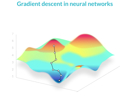{:.lead data-width="800" data-height="100"} Quotes from my students on why they are taking physics. {:.figure} ``` We solve for the weights and bias using an iterative method called "gradient descent". Plot the loss for a range of weights, for example. The plot should look like the image above. Our loss is minimized at the global minimum, much like the lowest point in a mountain range. The shortest path there is the steepest path. Given our currents weights and bias we look at all possible steps (e.g. up, down, left, right) and step in the direction with the steepest descent. This is calculated using partial derivatives. ```
By convention we typically refer to the loss function as the error for a simple training example and the cost function as the error for the batch of training examples. For example, the loss function could be the squared error and the cost function could the average squared error.
Gradient Descent
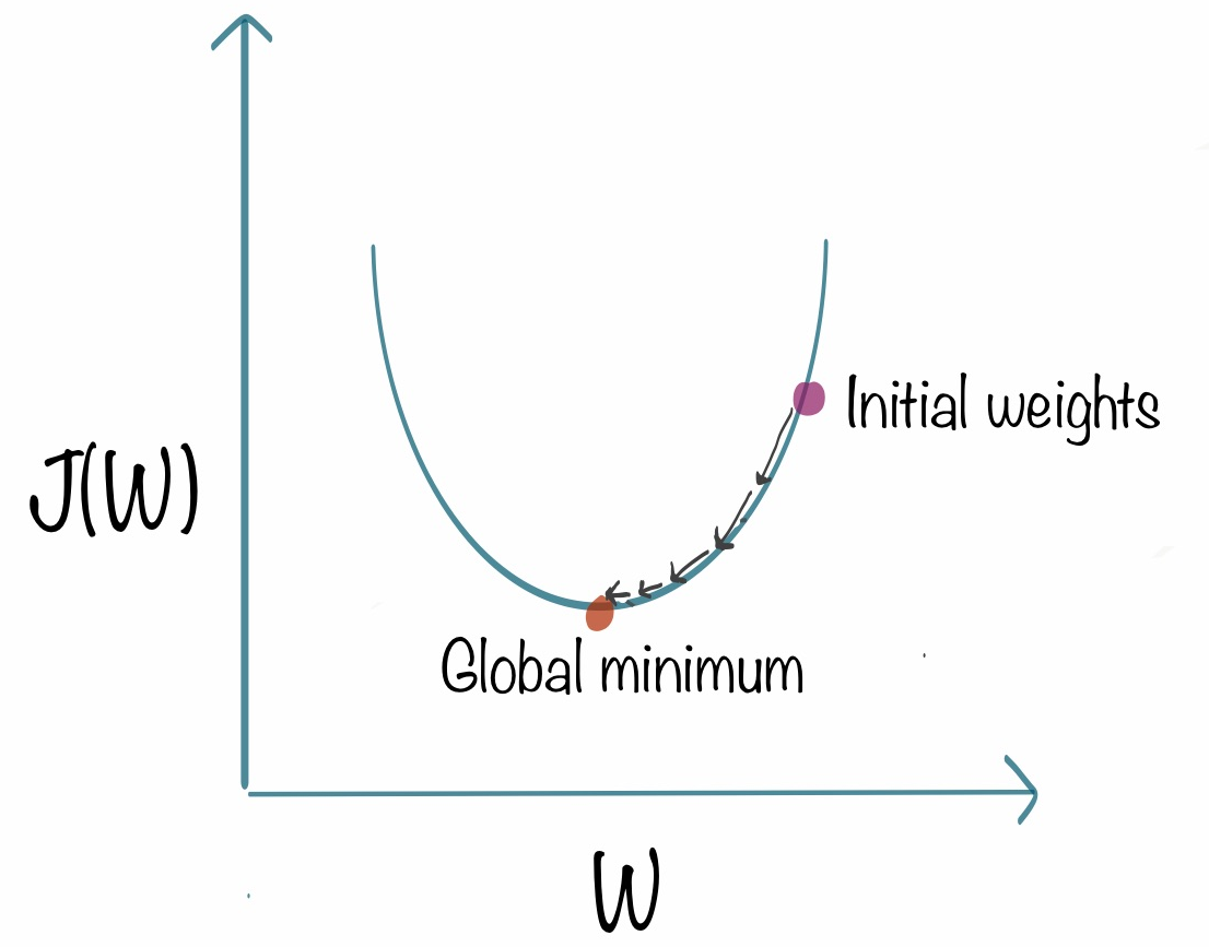
A plot the cost $J$ as a function of one weight $w$ might look like a parabola.
 Quotes from my students on why they are taking physics.
Any point to the left of the minimum has a negative slope and points towards the minimum. Any point to the right of the minimum as a postive slope and points away from the minimum. Therefore, the partial derivative of the cost function with respect to the weight can point us in the direction of the global minimum. \[\frac{\partial J}{\partial w}\]
and the weight should be updated by some amount of this partial derivative. This is our “alpha” term, which we call the learning rate. \[w = w-\alpha \frac{\partial J}{\partial w}\]
When the cost is left of the minimum the slope is negative. Thus, our new weight will be larger and the cost is lower. When the cost is right of the minimum our weight updates to a smaller value and the cost also lowers. And this same intuition applies for the bias, too! \[b = b-\alpha \frac{\partial J}{\partial b}\]
PSEUDO-ISH CODE
Example 1
# FOR ONE TRAINING EXAMPLE 'x' and label 'y'
# 3 LAYERS: 1 input layer, 1 hidden layer, 1 output layer
dz2 = a2-y
dw2 = dz2*a1.T
db2 = np.sum(dz2)
dz1 = w2.T*dz2*dg(z1) # dg is the derivative of the activation function
dw1 = dz1*x
db1 = np.sum(dz1)
w1 = w1 - alpha*dw1 # alpha is the learning rate
b1 = b1 - alpha*db1
w2 = w2 - alpha*dw2
b2 = b2 - alpha*db2
Your Turn - XOR Problem
Take what you’ve learned to re-implement the code for the XOR problem. REFERENCE
- 2 inputs: { \(x_1,x_2\) }
- 1 hidden layer with {2,3,4} neurons
- 1 output: $[0,1]$
Tasks
- Modify
__init__to account for the hidden layer weights and bias - Modify
forwardpropagation - Modify
backwardpropagation
Sample Class
# neural network with backprop
import numpy as np
import matplotlib.pylab as plt
%matplotlib inline

class Net():

    def __init__(self, layers=[input_layer,hidden_layer,output_layer]):
        np.random.seed(1) # for consistency
        self.w = # use list comprehension and np.random.uniform to create weights
        self.b = # use list comprehension and np.random.uniform to create bias

    def sigmoid (self, x):
        return 1/(1 + np.exp(-x))

    def sigmoid_derivative(self, x):
        return x * (1 - x)

    def forward(self, x):
        z0 = self.sigmoid(np.dot(x,self.w[0]) + self.b[0])
        z1 = # use sigmoid to forward propagate inputs
        return (z0, z1)

    def backward(self, inputs, z, labels, alpha):
        error = labels - z[1]
        d1 = error * self.sigmoid_derivative(z[1])
        d0 = d1.dot(self.w[1].T) * self.sigmoid_derivative(z[0])
        # update weights/biases
        self.w[1] += # use w[0] update as reference
        self.b[1] += # use b[0] update as reference
        self.w[0] += inputs.T.dot(d0) * alpha
        self.b[0] += np.sum(d0,axis=0,keepdims=True) * alpha

    def train(self, inputs, labels, epochs=100, alpha=0.1):
        errors = []
        for t in range(epochs):
            z = self.forward(inputs)
            self.backward(inputs, z, labels, alpha)
             # calculate loss (MSE)
            loss = np.mean((labels-z[1])**2)
            errors.append(loss)

        plt.plot(errors)
        plt.xlabel('epoch')
        plt.ylabel('loss (MSE)')
        plt.show()
Generating Data
import numpy as np
from sklearn.datasets import make_blobs
from sklearn.preprocessing import StandardScaler
plt.xkcd()
# Generate sample data
centers = [[1, 1], [-1, -1], [1, -1],[-1, 1]] # 4 centers
X, Y = make_blobs(n_samples=400, centers=centers, cluster_std=0.25,random_state=0)
# scale the X data
X = StandardScaler().fit_transform(X)
# reset labels
Y = np.array([1 if (YY == 3 or YY == 2) else 0 for YY in Y ])
# plot data
plt.figure(figsize=(16,12))
plt.rcParams.update({'font.size': 22,'font.family': ['Helvetica']})
plt.scatter(X[:,0], X[:,1], c=Y)
plt.xlabel('$x_1$')
plt.ylabel('$x_2$')
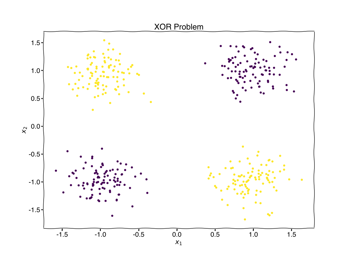
plt.title('XOR Problem')
plt.savefig('figure8.png')
plt.show()
Output
Split, Train, & Test
Use SKLearn to split your data,{ \(X,Y\)} into a training set and a testing set. Then use the Net() class to train on the data. Sample code provided below.
x_train, x_test, y_train, y_test = train_test_split(x, y, random_state=42) # split data
model = Net(layers=[2,4,1])
model.train(x_train,y_train.reshape(y_train.shape[0],1))
print(f'weights={model.weights} bias={model.bias}')
Here is a simple check for the XOR problem.
inputs = np.array([[-1,-1],[1,1],[-1,1],[1,0]])
labels = [0,0,1,1]

predictions = model.forward(inputs)[1]
predictions = [1 if prediction > 0.5 else 0 for prediction in predictions]

print("~~~ Results ~~~")
for item in zip(predictions,labels):
    print(item)


~~~ Results ~~~
(0, 0)
(0, 0)
(1, 1)
(1, 1)
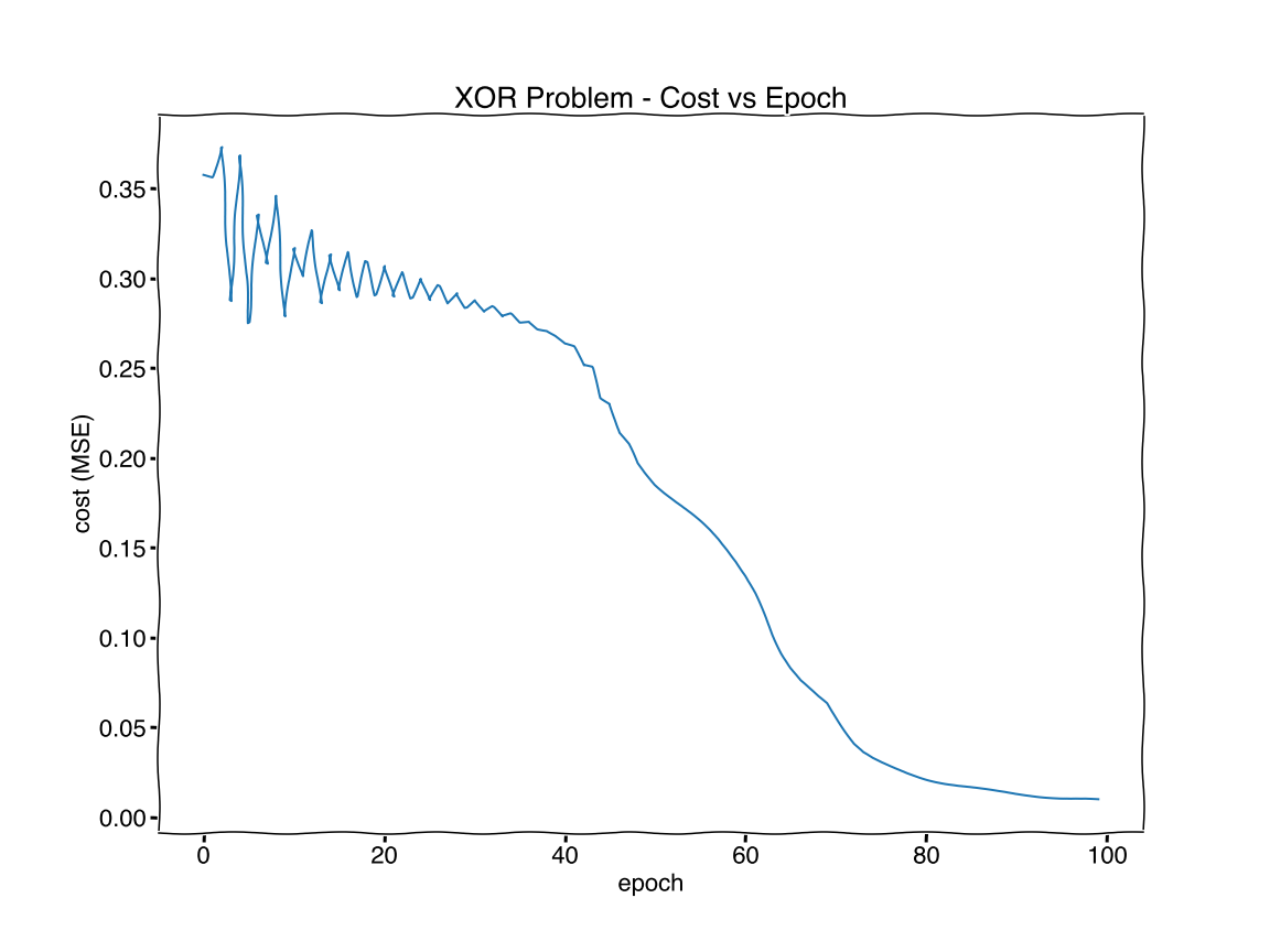
Cost vs Epoch
# neural network with backprop
import numpy as np
import matplotlib.pylab as plt
%matplotlib inline

class Net():

    def __init__(self, layers):
        np.random.seed(1) # for consistency
        self.w = [np.random.uniform(size=(layers[i], layers[i+1])) for i in range(len(layers)-1)]
        self.b = [np.random.uniform(size=(1, layers[i+1])) for i in range(len(layers)-1)]

    def sigmoid (self, x):
        return 1/(1 + np.exp(-x))

    def sigmoid_derivative(self, x):
        return x * (1 - x)

    def forward(self, x):
        z0 = self.sigmoid(np.dot(x,self.w[0]) + self.b[0])
        z1 = self.sigmoid(np.dot(z0, self.w[1]) + self.b[1])
        return (z0, z1)

    def backward(self, inputs, z, labels, lr):
        error = labels - z[1]
        d1 = error * self.sigmoid_derivative(z[1])
        d0 = d1.dot(self.w[1].T) * self.sigmoid_derivative(z[0])
        # update weights/biases
        self.w[1] += z[0].T.dot(d1) * lr
        self.b[1] += np.sum(d1,axis=0,keepdims=True) * lr
        self.w[0] += inputs.T.dot(d0) * lr
        self.b[0] += np.sum(d0,axis=0,keepdims=True) * lr

    def train(self, inputs, labels, epochs=100, lr=0.1):
        errors = []
        for t in range(epochs):
            # forward and backward propagation
            z = self.forward(inputs)
            self.backward(inputs, z, labels, lr)

             # calculate loss (MSE)
            cost = np.mean((labels-z[1])**2)
            errors.append(cost)

        # plot results
        plt.figure(figsize=(16,12))
        plt.rcParams.update({'font.size': 22,'font.family': ['Helvetica']})
        plt.plot(errors)
        plt.xlabel('epoch')
        plt.ylabel('cost (MSE)')
        plt.title('XOR Problem - Cost vs Epoch')
        plt.savefig('figure9.png')
        plt.show()


x_train, x_test, y_train, y_test = train_test_split(X, Y, random_state=42) # split data
model = Net(layers=[2,4,1])
model.train(x_train,y_train.reshape(-1,1))
print("\nWeights: ", model.w)
print("\nBias: ", model.b)
 Output
Weights:  [array([[ 2.85217211,  3.55374108, -1.81112541,  3.02762077],
       [ 2.93127264, -1.55898884,  3.68635881,  3.12471744]]), array([[-3.32488155],
       [ 5.23723096],
       [ 5.21112866],
       [-3.76024581]])]

Bias:  [array([[-3.76032457, -1.87048975, -2.07108773, -3.91527058]]), array([[-2.21562984]])]