A Brief History of the Electron
A brief history of the electron
Discovery of the Electron
Through the \(19^{th}\) century, matter was believed to be constructed of vast numbers of molecules, which are collections of atoms arranged in specific orientations. Atoms were believed to be the most fundamental component of matter, and were known to be electrically neutral. The word atom is derived from Greek atomos meaning indivisible. Thus, scientists believed there was no more fundamental unit of matter than the atom. At the time, physicist believed three fundamental forces governed the motion and interaction of all matter in the universe, down to the atom. The three fundamental forces were: gravity, electricity, and magnetism. In 1861, James Clerk Maxwell published a set of equations subsequently unifying electricity and magnetism into one fundamental force, the electromagnetic force [6]. \[\begin{aligned} \nabla \bullet \vec{E} &= \frac{\rho}{\varepsilon_{0}} \\[2em] \nabla \bullet \vec{B} &= 0 \\[2em] \nabla \times \vec{E} &= - \dot{\vec{E}} \\[2em] \nabla \times \vec{B} &= \mu_{0}\vec{J} + \mu_{0} \varepsilon_{0} \dot{\vec{E}} \end{aligned}\]
Eq. 1
In 1865, Maxwell showed that a charged object, simultaneously traversing external electric and magnetic fields, would “feel” the Lorentz Force \[\vec{F} = {\vec{F}}_{E} + {\vec{F}}_{B} = q\left( \vec{E} + \vec{v} \times \vec{B} \right)\]
Eq. 2
which is the sum of the electric force \({\vec{F}}_{E}\) and the magnetic force \({\vec{F}}_{B}\) [7]. During the years of 1895-1897 four major discoveries would lead to a new paradigm, the atomic age, which would inevitably show that Newton’s laws and Maxwell’s equations were not enough to describe all of nature.
The atomic age starts with the German physicist Wilhelm Roentgen studying the effects of cathode rays on various materials. In 1895 Roentgen noticed a nearby phosphorescent screen glowing even though it was not exposed to cathode rays [8]. Roentgen concluded that the screen must have been exposed to a new type of ray and called them “x-rays”— due to their unknown origin. Roentgen began to study the x-rays and noticed that they were unaffected by magnetic fields, unlike cathode rays. Roentgen’s wife placed her hand between the cathode ray tube and a fluorescent screen to produce the first x-ray image (see Figure 1). In 1901 Roentgen received the first Nobel Prize in Physics for his discoveries [9].
The next major discovery in the atomic age was that of radioactivity, by Henri Becquerel. In 1896 Becquerel was studying sunlight absorption of potassium uranyl sulfate, a uranium salt [11]. The salt was exposed to sunlight, wrapped in black paper, then set on a photographic plate. The experiment was seemingly a misfortune because of the overcast day, but a clear image emerged after developing the plates. Becquerel began to study the rays responsible for the image on that overcast day, and he discovered these new rays were affected by magnetic fields, just like cathode rays.
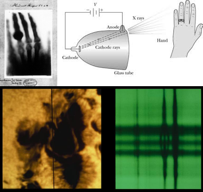 Figure 1 (a) Roentgen’s x-ray image of his wife’s hand. (b) Schematic of the setup of the cathode ray tube and the Roentgen’s wife’s hand. (c) Zeeman effect on a sunspot spectral line (Credit: NOAO/AURA/NSF) [10]. 8
Pierre and Marie Curie spent many years studying these new rays and referred to them as “radioactivity”. In honor of Becquerel, the International System (SI) of Units has termed the unit of radioactivity as the Becquerel (Bq) and is defined as one transformation (or decay or disintegration) per second [8], [12]. Becquerel shared the 1903 Nobel Prize in Physics with Pierre and Marie Curie “in recognition of the extraordinary services he has rendered by his discovery of spontaneous radioactivity” [12].
In 1896 Pieter Zeeman noticed the spreading of spectral lines when placing sodium under intense heat and in an external magnetic field. Zeeman’s findings were presented by Kamerlingh Onnes to the Dutch Academy of Sciences in October of 1897, with Henrik Antoon Lorentz present. Two days after the meeting, Lorentz proposed a theoretical model for the splitting by assuming atoms, believed to be the most fundamental unit of matter, contained charged particles called “ions” and these ions were to be harmonically bound to some central location [13]. Each frequency of oscillation was hypothesized to correspond to a spectral line. Therefore, the spreading should actually be distinct spectral line splitting. Lorentz’ theory follows.
An applied magnetic field \(\vec{H}\) in the \(\hat{z}\) direction should cause ions to experience a Lorentz force with corresponding equations of motion [13] \[\begin{aligned} m\ddot{x} &= - kx + \frac{\text{eH}}{c}\dot{y} \\[2em] m\ddot{y} &= - ky - \frac{\text{eH}}{c}\dot{x} \\[2em] m\ddot{z} &= - kz \end{aligned}\]
Eq. 3
having the general solutions \[\begin{aligned} x &= \{\begin{array}{c} a_1 \cos (\omega_1 t+p_1) \\ a_2 \cos (\omega_2 t+p_2) \end{array} \\[2em] y &= -a_1 \sin(\omega_1 t +p_1) \\[2em] z &= a \cos(\omega_0 t+p) \end{aligned}\]
Eq. 4
with the integration constants \(a\), phase constant \(p\), restoring spring constant \(k\), and frequencies \[\begin{aligned} \omega_{0} &= 2\pi\sqrt{k/m}, \\[2em] \omega_{0}^{2} &= \omega_{1}^{2} - \frac{\text{eH}}{\text{mc}}\omega_{1},\\[2em] \omega_{0}^{2} &= \omega_{2}^{2} + \frac{\text{eH}}{\text{mc}}\omega_{2}. \end{aligned}\]
Eq. 5
There will exist two circular motions in the \(x - y\) plane, one high and low frequency. There will be three linearly polarized components in total. Zeeman confirmed Lorentz’s theory on November 23, 1896 [14]. This spectral splitting is now referred to as the Normal Zeeman effect, and the 1902 Nobel Prize in Physics was awarded to Zeeman and Lorentz “in recognition of the extraordinary service they rendered by their research into the influence of magnetism upon radiation phenomena” [14], [15]. Study of the Zeeman effect has led to major advances in medical imagining known as magnetic resonance imaging (MRI), which is often used to image internal structures of biological subjects [16].
J.J. Larmor in 1897 derived the so-called Larmor formula which states that an accelerated charged object radiates energy in the form of electromagnetic waves [17], [18]. From Maxwell’s equations, it was also known that charged objects were affected by magnetic fields while electromagnetic waves were not. Roentgen’s experiment detected x-rays, which were not affected by magnetic fields, but the cathode rays within his experiment were. Additionally, Becquerel provided proof that another ray of unknown origin was also affected by magnetic fields— just like cathode rays. Finally, Zeeman and Lorentz provided mathematical and experimental proof of ions. In summary, the discovery of x-rays, radioactivity, and the Zeeman effect all hinted at the presence of a charged particle within matter.
In 1897 J.J. Thomson, a professor of physics at Cambridge University, sent cathode rays through external magnetic and electric fields to show that these rays behave as particles affected by both fields [19], [20]. Thomson also sent these charged particles through collimators and a combination of electric and magnetic fields to measure the deflection incurred by way of the Lorentz force. The experiment was intended to measure the charge-to-mass ratio of cathode rays. The ratio was determined to be \(\frac{q}{m} = 1.759×10^{11} C/kg\), and this ratio was concluded to be an absolute value—a constant [21]. Thomson quickly realized either the charge was large or the mass was small because these carriers of electricity were far more penetrating than molecules. Therefore, the molecules must be significantly larger than these carriers. G. Johnstone Stoney called these carriers of electricity as electrons [22].
In 1911 Robert A. Millikan determined the electron to carry a charge of \(q = -1.602×10^{-19} C \equiv - e\) [23]. Having the charge-to-mass ratio and the charge the electron mass follows as \(m_{e} = 9.109×10^{-31} kg\), a relatively small value, just as Thomson predicted. After the discovery of the electron, physicists were hoping to gain better insight into the inherent structure and physical properties of the electron. Let us consider the following thought experiment.
Suppose the electron is a sphere of infinitely many infinitesimal constituent pieces, then apply an external force to this structure. The external force adds motion to the electron, which adds momentum to anything inside, including a non-electromagnetic or mechanical mass. Now, suppose a charge is moving with uniform velocity through space \(v \ll c\). For some arbitrary point $P$ at some distance \(r\) and angle \(\theta\), with respect to $v$, the momentum density is given by [24] \[\vec{g} = \varepsilon_{0}\vec{E} \times \vec{B}.\]
Eq. 6
Knowing that the magnetic field is $B = v \times E/c^{2}$, we find the magnitude of the momentum density to be \[\left| \vec{g} \right| = \frac{\varepsilon_{0}v}{c^{2}}E^{2}\sin\theta.\]
Eq. 7
Since the fields are cylindrically symmetric about the line of motion, integration over all-space will reveal the transverse component to sum to zero. Therefore, the resultant momentum will be found to be parallel to the motion.
The total momentum is found by integrating Eq. 7 over all-space. Using the volume element \(d\mathcal{V} = 2\pi r^{2}\sin\theta\text{dθdr}\) and the transverse momentum component \(g_{T} = g\sin\theta\), the transverse momentum is \[{\vec{p}}_{T} = \int_{}^{}{\frac{\varepsilon_{0}v}{c^{2}}E^{2}\operatorname{}\theta}2\pi r^{2}\text{dθdr.}\]
Eq. 8
Here we choose to split the integral \[{\vec{p}}_{T} = \frac{\vec{v}}{c^{2}}\left( 4\pi\int_{R}^{\infty}\frac{\varepsilon_{0}E^{2}r^{2}}{2}\text{dr} \right)\left( \int_{0}^{\pi}{\operatorname{}\theta}\text{dθ} \right).\]
Eq. 9
The first integral can be recognized as the electron’s electric field energy, where the
energy density is given by \[w = \frac{\varepsilon_{0}}{2}\vec{E}\left( \vec{r} \right) \bullet \vec{E}\left( \vec{r} \right) = \frac{\varepsilon_{0}}{2}\left( \frac{q}{4\pi\varepsilon_{0}r^{2}} \right)^{2},\]
Eq. 10
and the electrostatic energy is found to be \[W_{E} = \int_{R}^{\infty}\frac{\varepsilon_{0}E^{2}r^{2}}{2} = 4\pi\frac{\varepsilon_{0}}{2}\left( \frac{- e}{4\pi\varepsilon_{0}} \right)^{2}\int_{R}^{\infty}{r^{- 2}\text{dr}} = \frac{1}{2}\frac{e^{2}}{4\pi\varepsilon_{0}R},\]
Eq. 11
where we have assigned spherical symmetry to an arbitrary radius $R$. The second integral of Eq. 9 is \[\int_{0}^{\pi}{\operatorname{}\theta}d\theta = - \int_{0}^{\pi}\left( 1 - \left( \cos\theta \right)^{2} \right)d\left( \cos\theta \right) = \left\lbrack - \cos\theta + \frac{\operatorname{}\theta}{3} \right|_{0}^{\pi} = \frac{4}{3}.\]
Eq. 12
Therefore, the transverse momentum follows as \[\vec{p}_{T} = \frac{1}{c^{2}} W_{E} \frac{4}{3} \vec{v} = \frac{1}{c^{2}} \frac{2}{3} \frac{e^{2}}{4\pi\varepsilon_{0}R} \vec{v} = m_{E}\vec{v}\]
Eq. 13
and we introduce the electromagnetic mass of the electron \(m_{E}\). In terms of the electromagnetic mass the self-energy of the electron can thus be written as \[W_{E} = \frac{3}{4}m_{E}c^{2}.\]
Eq. 14
This result was obtained classically and before Einstein introduced his famous equation \(W = m_{0}c^{2}\). It is possible to estimate the effective radius of the electron if one forces the two energies to be the same \[R = \frac{2}{3}a,\]
Eq. 15
where we have introduced the classical electron radius \[a = \frac{e^{2}}{4\pi\varepsilon_{0}m_{0}c^{2}}.\]
Eq. 16
In 1902 Abraham expanded on the above ideas by introducing an electron mass that is velocity dependent [25]. In his derivation, Abraham assumed the electron to be spherical and perfectly rigid (no deformation) and obtained for the transverse electron mass, in series form, to be \[m_{T}^{\left( \text{Abr} \right)} \cong \frac{2}{3}\frac{q^{2}}{4\pi\varepsilon_{0}Rc^{2}}\left( 1 + \frac{2}{5}\beta^{2} \right) + \ldots,\]
Eq. 17
where \(\beta \equiv v/c\). Lorentz, having published his work on length contractions in 1899, considered Abraham’s mass derivation and argued that an object in motion should experience deformation and undergo length contractions. In 1904 Lorentz re-derived the transverse mass [26] \[m_{T}^{\left( \text{Lor} \right)} \cong \frac{2}{3}\frac{q^{2}}{4\pi\varepsilon_{0}Rc^{2}}\left( 1 + \frac{1}{2}\beta^{2} \right) + \ldots.\]
Eq. 18
In the low velocity limit (\(\beta \rightarrow 0\)) the masses of Eq. 17 and Eq. 19 tend to \[\begin{aligned} m_{T}^{\left( \text{Abr} \right)} &\cong \frac{2}{3}\frac{q^{2}}{4\pi\varepsilon_{0}Rc^{2}}, \\[2em] m_{T}^{\left( \text{Lor} \right)} &\cong \frac{2}{3}\frac{q^{2}}{4\pi\varepsilon_{0}Rc^{2}}, \end{aligned}\]
Eq. 19
which is exactly the same as the mass term in Eq. 13. For an in-depth analysis of Abraham and Lorentz’s mass models see Jackson Ch.16 and Griffiths Ch.11 [27], [28].
In 1905 when Einstein published the special theory of relativity he also proposed the energy-mass equivalence, which was already well-studied [24], [25], [29]–[31] \[W = m_{0}c^{2}\sqrt{1 + \left( \frac{p}{m_{0}c} \right)^{2}}.\]
Eq. 20
In the stationary case where an object’s momentum is zero (\(p = 0\)) the energy reduces to \(W_{\text{tot}} = m_{0}c^{2}\). Returning to the mass relations above \[m_{0}c^{2} = W_{E}\frac{4}{3}\]
Eq. 21
or \[W_{\text{tot}} = W_{E}\frac{4}{3}\]
Eq. 22
or \[W_{E} = \frac{3}{4}W_{\text{tot}}.\]
Eq. 23
Clearly there is a missing energy of ¼ known as the “4/3-problem”. It should be noted that the geometry of the charge can be arbitrarily changed and only the factor of 4/3 would change to some other fraction. Therefore, it would be referred to as the “fraction-problem”. This discrepancy suggests that the relationship between the energy of a particle and its momentum differs between the classical laws of kinematics and electrodynamics. Moreover, the Einsteinian velocity dependent mass is a general consequence that is independent of an object’s structure whereas the Abraham and Lorentz models are geometry dependent. In 1905 Henri Poincare introduced the Poincare stresses as a form of non-electromagnetic pressure that holds the electron together such that \(W_{\text{tot}} = W_{E} + W_{M} = W_{\text{tot}} + W_{M}\), where \(W_{M} = W_{\text{tot}}/4\) is the mechanical energy associated with the Poincare stresses [24], [25], [27], [28], [31]. Poincare based the existence of these stresses on the following argument.
If the electron were purely electromagnetic in nature and it were broken into infinitely many infinitesimal units of charge, all of which exhibited coulombic forces, as each constituent electronic unit is brought together to build the electron the coulombic forces within the electron would be so great that the electron would explode. To prevent this explosion Poincare instituted his Lorentz invariant Poincare stresses. For a more complete and mathematically involved description of Poincare stresses see Jackson [28]. As Richard P. Feynman points out, if the electron has internal stresses it could oscillate or shake with modes which have yet to be observed [24]. These internal stresses may provide Lorentz-invariant stability to the electron but they introduce further complexities. Most significantly, the Poincare stresses provide an electron that reacts before acted on and has an inherent self-force that exponentially increases with time. It was also later shown that a relativistic reformulation of Eq. 9 resolves the incompatibility between Newton’s laws and electrodynamics.
Atomic Structure
Through the \(19^{th}\) century atoms (derived from Greek atomos meaning indivisible) were believed to be the most fundamental component of matter and were known to be electrically neutral. All known molecules were constructed with atoms and different atomic structures provided different molecules. The electron had no place in this worldview because atoms were indivisible. Therefore, the discoveries of the 1890s, most importantly the electron, indicated that the known laws, beliefs, and paradigm was incomplete. Thomson proposed various models of the atom to include electrons in a new world view [19].
Thomson reasoned atoms were comprised of equal positive and negative charge, where the source of negative charge was the electron (or many electrons). Having paired positive and negative charges allows for the atom to remain neutral while accounting for the inclusion of electrons. Thomson proposed the following three atomic models to account for this type of atomic structure and neutrality:
1) Each electron had an associated positively charged particle that it paired with.
2) Electrons orbited a central region of equal charge, similar to Lorentz’s model for the Normal Zeeman effect (as we will see, the Bohr model).
3) Evenly distributed electrons occupied a uniformly distributed, equally positive, charged region of space; termed the “plum pudding model”.
Thomson published his models in 1904 and chose the plum pudding model as the most likely [32]. In 1911 Ernest Rutherford completed his analysis of the 1908 Geiger-Marsden experiments, also known as the Rutherford gold foil experiments, where a beam alpha particles (positively charged; emitted through radioactivity; helium nucleus) were shot at a piece of gold foil and their scattering was measured in an attempt to probe the structure of the atom [33], [34]. If Thomson’s model was correct the beam would pass through the gold foil unobstructed because the atoms are uniformly neutral, but this result contradicts Rutherford’s experiment. The gold atom must consist of a densely packed nucleus of positive charge with electrons, much smaller than the nucleus, occupying some region beyond the nucleus.
Molecules were known to be extremely small, undetectable by the human eye, and atoms were believed to be much smaller than molecules. Rutherford’s experiment determined that electrons must be much smaller than the atom. Therefore, the electron not only has a small mass but it also has a small size.
Influences of Paul Dirac
Physics was conducted first by performing experiments then by finding mathematical formulations to support the empirical findings. Paul Dirac was the first to propose that physics could be done by “guessing” at the solutions, rather than waiting for experiment [35]. He believed that solutions could be found just by the elegance of the equations. Following these beliefs, in 1938 Dirac turned to the arguments of a moving charge [36].
For any object to accelerate there must be a force acting on it, but a force acting on an object will establish an imbalance of forces on the constituent parts. An imbalance within the electron would cause it to blowup because each differential charge would repel the others. For example, any two points within the electron, A and B, without acceleration, there exists some force \(F\). Adding all the forces between points in the electron and \(F = 0\).
Regarding Maxwell’s equation, for an emitter at position \(x_{0}\) and a receiver at \(x_{1}\), a signal leaves \(x_{0}\) and arrives at \(x_{1}\) at a later time, \(t_{r}\). This is known as the retarded solution, and it obeys causality, where signals propagate with a finite speed. However, there is also the advanced solution, for which the signal from \(x_{0}\) arrives at \(x_{1}\) at the time \(- t_{r}\). Generally, the advanced solution is disregarded as it is deemed unphysical and violates causality because a signal arriving at \(- t_{r}\) would be detected before it was emitted.
Using retarded potentials and considering an electron experiencing acceleration, the sum total force \(F \neq 0\). There is an imbalance because the force depends on the position of the points and the position depends time. The force is found to be \[F = \frac{e^{2}}{4\pi\varepsilon_{0}}\left\lbrack \alpha\frac{d^{2}x}{dt^{2}} - \frac{2}{3}\frac{1}{c^{3}}\frac{d^{3}x}{dt^{3}} + \beta\frac{d^{4}x}{dt^{4}} + \ldots \right\rbrack.\]
Eq. 24
The constants \(\alpha\) and \(\beta\) dependent on the geometry of the system used and are used for simplification. Dirac then calculated the same force using the advanced potentials. \[F = \frac{e^{2}}{4\pi\varepsilon_{0}}\left\lbrack \alpha\ddot{x} + \frac{2}{3}\frac{1}{c^{3}}\dddot{x} + \beta\frac{d^{4}x}{dt^{4}} + \ldots \right\rbrack\]
Eq. 25
He noticed that only the even-numbered derivative terms are geometry dependent. He eliminated these size dependent terms by assumed the net force to be the difference of half retarded and half advanced waves, for which the force becomes \[F = \frac{e^{2}}{4\pi\varepsilon_{0}}\left\lbrack \frac{2}{3}\frac{1}{c^{3}}\dddot{x} + higher\ terms \right\rbrack,\]
Eq. 26
where the higher terms of Eq. 26 contain powers of $a$, the classical electron radius, and in the limit of $a \rightarrow 0$ the above result should become model independent.
As Larmor derived decades earlier, an accelerating particle radiates energy in the form of electromagnetic waves [37]. Due to the loss of energy, the particle must “feel” a recoil or loss of momentum. The total power radiated of a non-relativistic particle (\(v \ll c\)) is given by \[P = \frac{e^{2}}{6\pi\varepsilon_{0}c^{3}}{\ddot{x}}^{2}.\]
Eq. 27
Suppose this particle is undergoing periodic motion such that its final state at $t_{2}$ is identical to its initial state at $t_{1}$, then the average power can be written as \[P = {\vec{F}}_{\text{rad}} \cdot \vec{v} \\ = \vec{F}_{\text{rad}} \cdot \frac{d}{\text{dt}}\left\lbrack \vec{x} \right\rbrack \\ = \frac{e^{2}}{6\pi\varepsilon_{0}c^{3}}{\ddot{x}}^{2}.\]
Eq. 28
The force term \({\vec{F}}_{\text{rad}}\) is interpreted as the force responsible for radiating. The radiation force can be calculated as \[\left| {\vec{F}}_{\text{rad}} \right| = \frac{e^{2}}{6\pi\varepsilon_{0}c^{3}}\dddot{x}.\]
Eq. 29
Dirac then conclude that the electron should be a point charge (\(a \rightarrow 0\)) to provide consistently between the reaction force and the radiation force. We now refer to the force as the radiation reaction. Dirac says this choice is “…not so much to get a model of the electron as to get a simple scheme of equations which can be used to calculate all the results that can be obtained from experiment,” [36]. With this assignment, Dirac’s point model saved classical theory through correspondence with radiation. Feynman also spent time working on the radiation reaction and gave a lecture on his analysis during the 1965 Nobel ceremonies [38].
Now that we have assigned the electron to be a point charge all of its energy must be stored within its fields. Taking the limit of Eq. 11 as the radius tends toward zero, just as Dirac’s point electron, the energy is \[\operatorname{}{W_{E}\left( a \right)} = \operatorname{}\frac{e^{2}}{8\pi\varepsilon_{0}a} \rightarrow \infty.\]
Eq. 30
We now see that a point charge has infinite self-energy; we have discovered the so-called electron self-energy paradox. Dirac would claim that the point electron is “not based on a model conforming to current physical ideas”; rather, chosen “to get a simple scheme of equations which can be used to calculate all the results that can be obtained from experiment,” [36]. The most current and accurate experiments find the electron radius to be \(a \leq 10^{- 18}\) m [39]. Therefore, for all intents and purposes, the electron seems to be a point charge.
Influences of Quantum Mechanics
At the turn of the century, in 1901, Max Planck explained black-body radiation, the spectral energy distribution of the radiation within an enclosure held at constant temperature (e.g. the sun), through the notion of atomic oscillators that have discrete rather than continuous distribution of energies [40]. Planck’s idea resolved the ultraviolet catastrophe and better predicted emission spectra of radiant objects. In 1905, Einstein published his theory of the photoelectric effect, the production of electrons caused by light incident on a material, for which he later won the 1921 Nobel Prize in Physics [41], [42]. Einstein proposed that light traveled in discrete wave packets of energy called photons. Verification of the photoelectric effect provided secondary validation of the energy discretization, which was used by Niels Bohr to propose a new atomic model.
Building on the ideas of quantization and Rutherford’s conclusions of the atom, in 1913 Bohr proposed three ansatzes for the atom [43].
1) Electrons orbit the positively charged nucleus.
2) Electrons can only revolve around the nucleus in stable orbits, without radiating.
3) Electrons can only gain or lose energy by moving from one stable orbit to another.
Bohr was able to calculate the energy between the orbits by requiring the orbiting electron to have angular momentum of integer multiples, \(L = n\hslash,\ \ n \in \mathbb{Z}^{+}\). The spectra of the hydrogen atom were used to test Bohr’s model, for which his model was then shown to precisely predict the spectra for atoms of single electrons. After higher resolution spectroscopes were developed, more precise experiments showed limitations with the Bohr model. In summary,
1) Success with single electron atoms (e.g. \(H, He^+, Li^{++}\)),
2) Could not account for spectral line splitting,
3) Could not explain molecular binding.
Nevertheless, Bohr’s model was successful in showing quantization of the electron’s orbital angular momentum.
In 1915, Alfred Lauck Parson developed a spinning ring electron model that would explain the bonds between molecules as a consequence of two molecules sharing an electron [44]. Parson’s theory received attention from the respected Arthur Compton, but the theory quickly defaulted to the advances of quantum mechanics.
In the 1920s quantum mechanics was nearly fully developed and resolved the limitations the previous models. One of the most foundational experiments of the 1920’s for quantum mechanics and the development of the electron was the Stern-Gerlach experiments, which were intended to test the Bohr-Sommerfeld hypothesis, quantization of angular momentum, and were based on the Bohr model of the atom [45], [46]. An electron orbiting a central nucleus establishes a magnetic moment \[\begin{aligned} \mu &= A \bullet I \\[2em] &= \pi r^{2}I \\[2em] &= \pi r^{2}\frac{q}{T}\\[2em] &= \pi r^{2}\frac{\text{qv}}{2\pi r} \\[2em] &\equiv \frac{q}{2mc}L \end{aligned}\]
Eq. 31
where \(L\) is the orbital angular momentum of the particle. The beam was sent through an initial magnetic field, then sent through a filter to achieve a “pure” beam of with magnetic moments in the same direction. They then sent the filtered beam through various combinations of magnetic fields. Through this series of experiments Stern and Gerlach determined that there is some unaccounted for angular momentum.
George Uhlenbeck and Samuel Goudsmit analyzed spectral splitting of the hydrogen atom in an effort to develop a novel theory to explain said splitting [47]. Eventually they showed that the spectral splitting could be accounted for if the electron were a spinning sphere. Their advisor Paul Ehrenfest sent the two men to discuss their model with Lorentz. Lorentz then showed them that the electron must be spinning approximately an order of magnitude larger than the speed of light, \(\frac{v}{c} \approx 137 = 1/\alpha\). Ehrenfest had already sent their theory for publication in 1926 by the time Goudsmit and Uhlenbeck informed Ehrenfest of their foolishness. Ehrenfest was quoted, “…both [are] young enough to be able to afford a stupidity” [48]. Nevertheless, we refer to the electron’s intrinsic angular momentum as spin because of their theory.
During the 1940s it was known that quantum mechanics could not sufficiently predict the electron’s magnetic moment [49]. Experiments were showing that there was some “anomalous” correction to the electron’s magnetic moment. To avoid the singularities of classical electrodynamics and to explain the anomalous magnetic moment, Sin-Itiro Tomonage, Julian Schwinger, and Richard P. Feynman were unknowingly, simultaneously working on the same quantum description of electrodynamics. QED predicted the electron’s magnetic moment to be \[\mu = \mu_{0}\left( 1 + \frac{\alpha}{2\pi} + \ldots \right),\]
Eq. 32
which proved to agree with experiment to great precision [50]–[52]. Current experimental values indicate QED’s theoretical prediction of the anomalous magnetic moment (\(\alpha/2\pi\)) to an accuracy of 1 part in 1 trillion. To date QED has been the most successful theory in physics, if not all of science. As I wrote earlier, what is the necessity to pursue a different model of the electron when the point charge has led to great success with QED? To answer, I quote Feynman summarizing QED [53].
“It seems that very little physical intuition has yet been developed I this subject. In nearly every case we are reduced to computing exactly the coefficient of some specific term. We have no way to get a general idea of the result to be expected. To make my view clearer, consider, for example, the anomalous electron moment…We have no physical picture by which we can easily see that the correction is roughly \(\alpha/2\pi\); in fact, we do not even know why the sign is positive (other than by computing it)…We have been computing terms like a blind man exploring a new room, but soon we must develop some concept of this room as a whole, and to have some general idea of what is contained in it. As a specific challenge, is there any method of computer the anomalous moment of the electron which, on first rough approximation, gives a fair approximation to the \(\alpha\) term?”
QED, even with its great success, never addressed the paradox of the point charge—it only circumvented it through mass renormalization. The infinities that emerge in QED also emerge in classical electrodynamics. Therefore, the necessity to pursue another model of the electron stems from the lack of classical understanding [38]. Our goal is to seek a deeper understanding of the electron and the corrections provided by QED by developing a classical renormalization procedure.
References
[1] H. Wilson, “An Electromagnetic Theory of Gravitation,” Phys. Rev., vol. 17, no. 1, pp. 54–59, Jan. 1921.
[2] R. Dicke, “Gravitation without a Principle of Equivalence,” Rev. Mod. Phys., vol. 29, no. 3, pp. 363–376, Jul. 1957.
[3] K. Krasnov, “Plebanski Formulation of General Relativity: A Practical Introduction,” p. 13, Apr. 2009.
[4] H. E. Puthoff, “Polarizable-Vacuum (PV) representation of general relativity,” arXiv Prepr. gr-qc/9909037, pp. 1–24, Sep. 1999.
[5] S. M. Blinder, “Structure and self-energy of the electron,” Int. J. Quantum Chem., vol. 90, no. 1, pp. 144–147, Aug. 2002.
[6] J. C. Maxwell, “On Physical Lines of Force,” Philos. Mag., vol. 4, 1861.
[7] J. C. Maxwell, “A Dynamical Theory of the Electromagnetic Field [J],” Philos. Trans. R. Soc. London, vol. 155, no. January, pp. 459–512, 1865.
[8] S. T. Thornton and A. Rex, Modern Physics for Scientists and Engineers, Revised. Saunders College, 1993.
[9] Nobel Media AB 2014, “The Nobel Prize in Physics 1901,” Nobelprize.org, 2016.
[10] NSO, AURA, and NSF, “Sunspot with Spectrum,” NOAO.EDU. [Online]. Available: https://www.noao.edu/image_gallery/html/im0404.html. [Accessed: 06-Jun-2016].
[11] R. A. Serway, C. J. Moses, and C. A. Moyer, Modern Physics, Third. Cengage Learning, 2004.
[12] Nobelprize.org, “Henri Becquerel - Facts.” [Online]. Available: https://www.nobelprize.org/nobel_prizes/physics/laureates/1903/becquerel-facts.html.
[13] A. Kox, “The discovery of the electron: II. The Zeeman effect,” Eur. J. Phys., vol. 18, pp. 139–144, 1997.
[14] Nobelprize.org, “Pieter Zeeman - Biographical,” Nobel Media AB 2014. [Online]. Available: http://www.nobelprize.org/nobel_prizes/physics/laureates/1902/zeeman-bio.html. [Accessed: 07-May-2016].
[15] Nobelprize.org, “The Nobel Prize in Physics in 1902,” Nobel Media AB 2014. [Online]. Available: http://www.nobelprize.org/nobel_prizes/physics/laureates/1902/. [Accessed: 07-May-2016].
[16] G. Kauffman, “Nobel Prize for MRI Imaging Denied to Raymond V. Damadian a Decade Ago,” Chem. Educ., vol. 4171, no. 14, pp. 73–90, 2014.
[17] H. Goldstein, C. P. Poole, and J. L. Safko, Classical Mechanics, Third. Pearson, 2001.
[18] J. Powell and B. Crasemann, Quantum Mechanics. London: Addison-Wesley Publishing Company, Inc, 1961.
[19] J. J. Thomson, Notes on Recent Researches in Electricity and Magnetism: Intended as a Sequel to Professor Clerk-Maxwell’s Treatise on Electricity and Magnetism. London: Oxford, The Clarendon Press, 1893.
[20] J. Thomson, “Cathode Rays,” Philosophical Magazine, vol. 44, p. 293, 1897.
[21] “Electron Charge to Mass Quotient,” NIST.gov. [Online]. Available: http://physics.nist.gov/cgi-bin/cuu/Value?esme. [Accessed: 07-Jun-2016].
[22] G. J. Stoney, “Of the ‘Electron’ or Atom of Electricity,” Philos. Mag., vol. 38, no. 5, pp. 418–420, 1894.
[23] R. A. Millikan, “The isolation of an ion, a precision measurement of its charge, and the correction of Stokes’s law,” Phys. Rev. (Series I), vol. 32, no. 4, pp. 349–397, 1911.
[24] R. P. Feynman, R. Leighton, and M. Sands, Feynman lectures on Physics, Volume II. California Institute of Technology, 1963.
[25] M. Janssen and M. Mecklenburg, “From Classical to Relativistic Mechanics: Electromagnetic models of the electron,” Interact. Math. Phys. Philos. 1860-1930, pp. 65–134, 2006.
[26] H. A. Lorentz, “Electromagnetic Phenomena in a System Moving with any Velocity Smaller than that of Light,” in Collected Papers, Dordrecht: Springer Netherlands, 1937, pp. 172–197.
[27] D. J. Griffiths, Introduction to Electrodynamics, Third. Prentice Hall, 1999.
[28] J. D. Jackson, Classical Electrodynamics, Third. Wiley, 1998.
[29] P. Acuna, “On the empirical equivalence between special relativity and Lorentz’s ether theory,” Stud. Hist. Philos. Sci. Part B - Stud. Hist. Philos. Mod. Phys., vol. 46, no. 1, pp. 283–302, 2014.
[30] A. Einstein, “on the Electrodynamics of Moving Bodies,” pp. 1–31, 1905.
[31] H. Poincare, “Sur la dynamique de l’electron,” Comptes Rendus l’Academie des Sci., vol. 140, no. 2, pp. 1504–1508, 1905.
[32] J. Thomson, “On the Structure of the Atom,” Philos. Mag., vol. 7, no. 39, pp. 237–265, 1904.
[33] E. B. Podgorsak, “3 Rutherford-Bohr Model of the Atom,” in Radiation Physics for Medical Physics, 2010, pp. 139–175.
[34] E. Rutherford, “The scattering of α and β particles by matter and the structure of the atom,” Philos. Mag., vol. 92, no. 4, pp. 379–398, 1911.
[35] R. P. Feynman and S. Weinberg, Elementary Particles and the Laws of Physics. Cambridge University Press, 1999.
[36] P. A. M. Dirac, “Classical Theory of Radiating Electrons,” Proc. R. Soc. A Math. Phys. Eng. Sci., vol. 167, pp. 148–169, 1938.
[37] J. Larmor, “LXIII. On the theory of the magnetic influence on spectra; and on the radiation from moving ions,” Philos. Mag. Ser. 5, vol. 44, no. 271, pp. 503–512, Dec. 1897.
[38] Nobel Media AB 2014, “Richard P. Feynmn - Nobel Lecture: The Development of the Space-Time View of Quantum Mechanics”,” Nobelprize.org, 1965. [Online]. Available: http://www.nobelprize.org/nobel_prizes/physics/laureates/1965/feynman-lecture.html. [Accessed: 06-Jun-2016].
[39] D. Bender, et al, “Tests of QED at 29 GeV center-of-mass energy,” Phys. Rev. D, vol. 30, no. 3, pp. 515–527, Aug. 1984.
[40] M. Planck, “On the law of the energy distribution in the normal spectrum,” Ann. Phys, vol. 4, pp. 1–11, 1901.
[41] Nobel Media AB 2014, “The Nobel Prize in Physics 1921,” Nobelprize.org. [Online]. Available: http://www.nobelprize.org/nobel_prizes/physics/laureates/1921/. [Accessed: 07-May-2016].
[42] A. Einstein, “On a Heuristic Point of View about the Creation and Conversion of Light?,” Ann. Phys., vol. 17, no. 132, p. 91, 1905.
[43] N. Bohr, “I. On the constitution of atoms and molecules,” London, Edinburgh, Dublin Philos., vol. 26, no. 777306420, pp. 1–25, 1913.
[44] A. L. Parson, “A magneton theory of the structure of the atom,” Smithson. Misc. Collect., vol. 65, pp. 1–80, 1915.
[45] J. J. Sakurai, “Modern Quantum Mechanics,” American Journal of Physics, vol. 54, no. 7. p. 668, 1994.
[46] J. S. Townsend, A Modern Approach to Quantum Mechanics. University Science Books, 2000.
[47] G. E. Uhlenbeck and S. Goudsmit, “Spinning Electrons and the Structure of Spectra,” Nature, vol. 117, no. 2938, pp. 264–265, Feb. 1926.
[48] G. E. Uhlenbeck, “Fifty Years of Spin: Personal reminiscences,” Phys. Today, vol. 29, no. 6, p. 43, 1976.
[49] J. E. Nafe, E. B. Nelson, and I. I. Rabi, “The Hyperfine Structure of Atomic Hydrogen and Deuterium,” Phys. Rev., vol. 71, no. 12, pp. 914–915, Jun. 1947.
[50] J. J. Sakurai, Advanced Quantum Mechanics. Addison-Wesley, 1967.
[51] J. Schwinger, “Quantum electrodynamics. III. The electromagnetic properties of the electron-radiative corrections to scattering,” Phys. Rev., vol. 76, no. 6, pp. 790–817, 1949.
[52] J. Schwinger, “On Quantum-Electrodynamics and the Magnetic Moment of the Electron,” Phys. Rev., vol. 73, no. 4, pp. 416–417, Feb. 1948.
[53] R. P. Feynman, “The Quantum Theory of Fields,” in Proceedings of the Twelfth Conference on Physics at the University of Brussels, 1961.
[54] W. Heisenberg, “Uber quantentheoretische Umdeutung kinematischer und mechanischer Beziehungen.,” Zeitschrift fur Phys., vol. 33, no. 1, pp. 879–893, Dec. 1925.
[55] J. A. Wheeler and W. H. Zurek, Quantum Theory Measurement. Princeton University Press, 2014.
[56] A. Sommerfeld and I. Runge, “Anwendung der Vektorrechnung auf die Grundlagen der Geometrischen Optik,” Ann. derk Phys., vol. 35, pp. 277–299.
[57] E. Schrodinger, “Collected Papers on Wave Mechanics.” Chelsea Publishing, New York, 1982.
[58] J.-H. Kim and H.-W. Lee, “Canonical transformations and the Hamilton-Jacobi theory in quantum mechanics,” Can. J. Phys., vol. 77, no. 6, pp. 411–425, Oct. 1999.
[59] R. S. Bhalla, “Quantum Hamilton–Jacobi formalism and the bound state spectra,” Am. J. Phys., vol. 65, no. 12, p. 1187, 1997.
[60] R. A. Leacock and M. J. Padgett, “Hamilton-Jacobi/action-angle quantum mechanics,” Phys. Rev. D, vol. 28, no. 10, pp. 2491–2502, Nov. 1983.
[61] D. Bohm, “A Suggested Interpretation of the Quantum Theory in Terms of ‘Hidden’ Variables. I,” Phys. Rev., vol. 85, no. 2. pp. 166–179, 1952.
[62] P. Jordan and E. Wigner, “Uber das Paulische Aquivalenzverbot,” Zeitschrift fur Phys., vol. 47, no. 9–10, pp. 631–651, 1928.
[63] P. Jordan and O. Klein, “Zum Mehrkorperproblem der Quantentheorie,” Zeitschrift fur Phys., vol. 45, no. 11–12, pp. 751–765, 1927.
[64] P. A. M. Dirac, “The Quantum Theory of the Emission and Absorption of Radiation,” Proc. R. Soc. A Math. Phys. Eng. Sci., vol. 114, no. 767, pp. 243–265, Mar. 1927.
[65] J. von Neumann, Mathematische Grundlagen der Quantenmechanik, vol. 42, no. 4. 1935.
[66] E. Wigner, “On the quantum correction for thermodynamic equilibrium,” Phys. Rev., vol. 40, no. 5, pp. 749–759, 1932.
[67] R. P. Feynman, “Space-time approach to non-relativistic quantum mechanics,” Rev. Mod. Phys., vol. 20, no. 2, pp. 367–387, 1948.
[68] E. Schrödinger, “Quantisierung als Eigenwertproblem,” Ann. Phys., vol. 385, no. 13, pp. 437–490, 1926.
[69] W. Heisenberg, “Uber den anschaulichen Inhalt der quantentheoretischen Kinematik und Mechanik,” Zeitschrift fur Phys., vol. 43, no. 3–4, pp. 172–198, Mar. 1927.
[70] B. L. van der Waerden, “Sources of Quantum Mechanics,” American Journal of Physics, 1968. [Online]. Available: http://store.doverpublications.com/048645892x.html.
[71] D. F. Styer, et al, “Nine formulations of quantum mechanics,” Am. J. Phys., vol. 70, no. 3, p. 288, 2002.
[72] P. Dirac, “The Quantum Theory of the Electron,” Proc. R. Soc. London. Ser. A, vol. 117, no. 778, pp. 610–624, 1928.
[73] G. Breit, “Dirac’s equation and the spin-spin interactions of two electrons,” Phys. Rev., vol. 39, no. 4, pp. 616–624, 1932.