Grad School Projects - Fractals
This work was for Statistical Mechanics
Authors
Neal Blackman
Raj Vinnakota
Brandon Touchet
Introduction
Fractals are never ending complex patterns that are self-similar, iterative, mathematical structures. For any general fractal iterating a set of “rules” that generate repeated structures on ever-smaller dimensions can generate its unique shape. For example, Figure 1 depicts a fern found in nature that can be mathematically redrawn to provide the same general image. In general, fractals can be deterministic (explained at the end of the report) or statistical in nature, and can be found everywhere in nature such as tree and leaf grow, blood vessels, neuron, lightening, and coastlines.
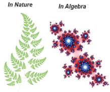 Figure 1. Two fractals, one commonly found in nature, that can be mathematically drawn
Reviewing different fractal-like images only perpetuates confusion and ambiguity when defining a fractal. For example, dendritic growth (or lightening) can seem to form randomly, but they do in-fact follow rules that give them iterative, self-similarity that is infinitely magnifiable. The difference between this type of pattern and more self-similar structure of a fern, cauliflower, or the Mandelbrot Set arises from the implementation of randomness— such randomness can be seen in snowflakes.
As ubiquitously recognized as all snowflakes are they are, all snowflakes are intrinsically unique. Their uniqueness is a consequence of a subtle implementation of randomness by nature. For example, Figure 2 illustrates a section of the famous Koch Snowflake. The Koch Snowflake can be form by starting with a line, or any closed polygon, and creating three equal parts of every straight line-segment. The middle section of line-segment trio is reshaped into an open triangle. By infinitely repeating this process with each original line-segment the Koch Snowflake can form.
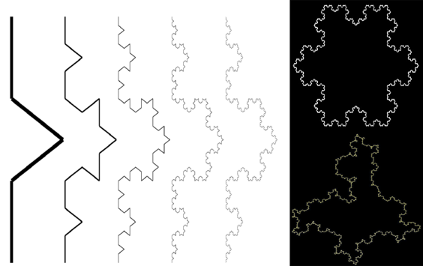 Figure 2. (LEFT) The Koch Snowflake through five iterations, with the zeroth iteration being a straight line. Properties: No. of Sides: \(N_{i+1} = 4N_i \rightarrow N_j=3(4^j)\), Length of the \(i^{th}\) side: \(L_{i+1} = L_i/3 \rightarrow L_j = (1/3)^jL_0\), Perimeter length (after the \(i^{th}\) iteration): \(P_j = N_j L_j = (4/3)^j L_0 \rightarrow \infty\), Total Area: \(A_j \rightarrow 1.6A_0\) (TOP RIGHT) Show the Koch Snowflake with each triangle forming on the outside. (BOTTOM RIGHT) Shows the Koch Snowflake by randomly choosing inside or outside
To implement randomness imagine changing the direction of the new triangles: let each new open triangle be formed on the inside or the outside of the original shape. The bottom right image in Figure 2 shows one variation of the randomness. We can imagine how to form intricate snowflakes including this type of randomness by having more symmetric rules in addition to more rules in general. Nature implements this randomness in other places as well. For example, dendritic growth, lightening, and molecular growth can be seen with similar fractal processes, which include elements of randomness.
Techniques
Iterated function systems – This techniques uses fixed geometric rules which may be stochastic e.g., Koch snowflake
Strange attractors – This technique uses iterations of a map of a system of initial-value differential equations that exhibit chaos.
Escape-time fractals – This technique uses a formula that’s being used recursively in the dimensional space. e.g., the Mandelbrot set.
Random fractals – This technique uses the stochastic rules; e.g., percolation clusters, trajectories of Brownian motion and the Brownian tree (i.e., dendritic fractals).
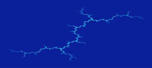
Dendritic growth can be achieved by forming a closed boundary with an arbitrarily placed seed position. Next, let an arbitrary amount of walkers move throughout the boundary until the walkers satisfy defined sticking conditions. Note, the walkers should not walk from the seed position. The walkers must start from a position that is not guaranteed to be on or next to the seed position. For example, the walkers may start from the boundary and the seed position may be the center of the geometry. If the walkers are built from the seed position, and not to the seed position, the object with form in a clumping manner, and cloud-like images will form.
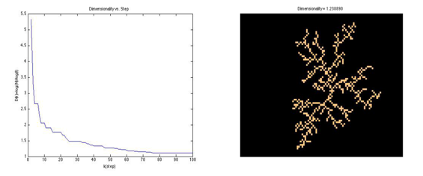 (LEFT) Shows that our object asymptotically reaches a finite dimensionality. For our given boundary conditions, our fractal objects (RIGHT) consistantly approached dimensionality near the dimensionality deterministic version.
Applications of fractals in modern sciences include, but are not limited to the following: weather forecasting, human anatomy, data compression, cloud and coastline measurement, astro-physics modeling, contemporary antennas, computer graphics, transistors, and iris recognition.
Researchers at Oregon state university developed a computer chip cooling systems which resembles like the fractal branches. This uses liquid nitrogen to as the cooling agent for the processor cooling. Fractal antennas is developed which has the ability to receive/tune to radio signals of a range of frequencies. These antennas have potential applications in cell-phones. Space filling Fractals are designed, which has the potential application as a mixer in the micro channel laminar flow of the fluid.
To further explore fractals, we further explored deterministic fractals by implementing the escape-time method. Deterministic fractals are fractals that would always reproduce the same image. Deterministic fractals are more purely and appropriately mathematical and significantly less natural due to their inherent exactness.
The Mandelbrot Set can be created by establishing a domain space, {X,Y}, then define a function some function to act on the space, Z({X,Y}). Define another function, F(Z), to act on the first function. Then, with each iteration shift Z by some constant. After a sufficient amount of iterations plot a gradient of the new domain space. So, the system would resemble something like the following: \(\begin{aligned} Z &= X+iY; \\ C &= -i; \\ for i &= 1:k \\ Z &= F(Z) + C; \\ end \\ colormap(e^{-|Z|}) \\ \end{aligned}\)
We used this process to define a deterministic dendrite of comparable size to compare the dimensionality, \(D = \frac{log N}{log l}\), with the statistical process, where \(N\) is the number of molecules used to build the fractal and is the length of the longest side of the bounding rectangle. Our statistical approach is near the deterministic approach. With further programming improvements and a better dimensionality definition our results should approach each other.
 Weakly interacting gas at high temperature. b) The atoms can be regarded as wave packets with an extension of their de Broglie wavelength \(λ_db\). c) At \(T<T_c\) the matter waves of each individual atom overlaps and \(λ_db\) is comparable to the inter-atomic distance and approaching the BEC state. d) At \(T<T_c\) the sea of wave packets disappears and behaves like single matter wave giving rise to the BEC.
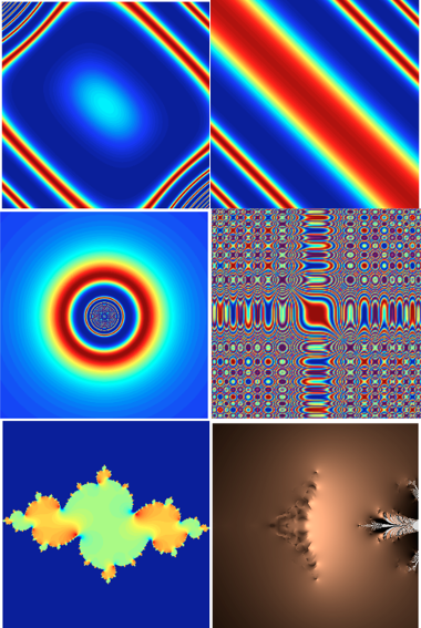
Example Art
Here is some fractal are. For the functions and constants used reference the Matlab code.
 Weakly interacting gas at high temperature. b) The atoms can be regarded as wave packets with an extension of their de Broglie wavelength \(λ_db\). c) At \(T<T_c\) the matter waves of each individual atom overlaps and \(λ_db\) is comparable to the inter-atomic distance and approaching the BEC state. d) At \(T<T_c\) the sea of wave packets disappears and behaves like single matter wave giving rise to the BEC.