Grad School Projects - Einstein Solid
This work was for Statistical Mechanics
Authors
- Neal Blackman
- Brandon Touchet
- Rajkumar Vinnakota
Random Configurations (Problem 1)
Methodology
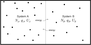
A system was configured with two solids: solid A with \(N_A\) oscillators and solid B with \(N_B\) oscillators. Each random configuration was generated by distributing a fixed total amount of energy, \(q_T\), to randomly selected oscillators. This was done by assigning each quantum of energy, \(q_i\), a random integer, \(n_i = 𝑅𝑎𝑛𝑑𝑜𝑚[1, 𝑁_A + 𝑁_B]\). For \(1 \leq 𝑛_i \leq 𝑁_A\), \(q_i\) was attributed to solid A; for \(𝑁_A < 𝑛_i ≤ 𝑁_A+N_B\), \(𝑞_i\) was attributed to solid B. This gives each oscillator equal weight, so the probability of assigning \(q_i\) to solid A or solid B is \[\begin{align} P(q_i \rightarrow q_A) &=\frac{N_A}{N_A+N_B} \\[2em] P(q_i \rightarrow q_B) &=\frac{N_B}{N_A+N_B} \\ \end{align}\]
Each configuration generated gives a pair of values, \({q_A,a_B}\), making \(𝑞_A\) and \(𝑞_B\) discrete random variables that follow the inherent probability distribution of the system. However, this algorithm implicitly assumes distinguishable \(𝑞_i\), contradicting the physical properties of energy. To see why this is so, consider Table 1. In this simple example, \(N_A=1\), \(N_B=1\), and \(𝑞_T=2\). If the \(q_i\) were distinguishable, there would be two states with \(a_A=1\), but there is only one such state for indistinguishable \(q_i\). To avoid overcounting microstates, we incorporate a correction factor. The correction factor counts the number of ways that distinguishable quanta can be distributed in a particular microstate. Using \(N_T=N_A+N_B\), the correction factor is \[CorrectionFactor = ( \frac{q_T!}{\prod^{N_T}_{i=1} q_i})^{-1}\]
As seen in Figure 1a, the unadjusted frequency for \(q_A=1\) is too high. The histogram that includes the correction factor, Figure 1b, matches the exact histogram, Figure 1c.
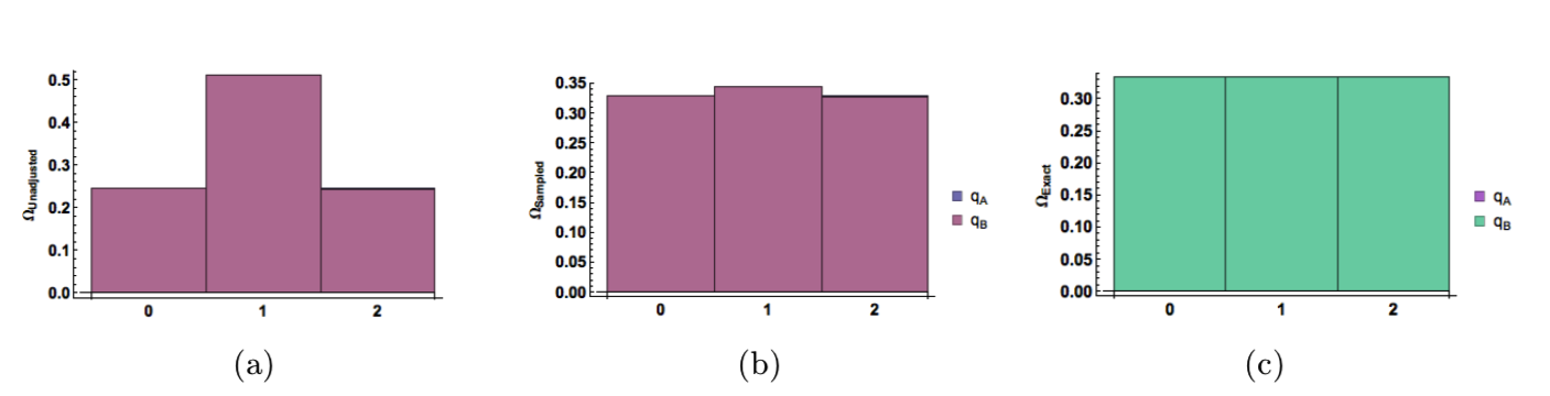 Figure 1: Demonstration of overcounting with \(𝑁_A = 1, 𝑁_B = 1,\) and \(𝑞_T = 2\). Normalized histograms are shown (a) without the correction factor, (b) with the correction factor, and (c) as given by the binomial distribution.
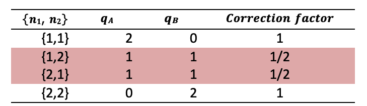 Table 1: Example of overcounting using random number generation. The highlighted rows correspond to the same macrostate for indistinguishable energy and should only be counted once.
Analytical Properties
We consider the properties of the system analytically to confirm the validity of our simulated results. We define the multiplicity of each macrostate to be \(\Omega_{AB}\) where \[\begin{equation} \Omega_{AB} \equiv \Omega_A \Omega_B = \binom{q_A+N_A-1}{q_A}\binom{q_B+N_B-1}{q_B} \end{equation}\]
Figure 2 shows a plot of \(\Omega_A\), \(\Omega_B\), and \(\Omega_{AB}\) for \(N_A=300\), \(N_A=200\), and \(q_T=300\). The probability of the system being in a particular state is \[\begin{equation} P_j= \frac{ \Omega_{AB} ({q_A,q_B}_j)}{\Sigma_{q_A,q_B} \Omega_{AB} ({q_A,q_B})} =\frac{\Omega_{AB} ({q_A,q_B}_j)}{ \Omega_{system}} \end{equation}\]
where \(\{q_A,q_B\}\) is the set of all possible macrostates that have \(q_A+a_B=q_T\), and \(\{q_A,q_B\}_j\) is one such macrostate. The sum in the denominator is just the multiplicity of the entire system, i.e. \[\begin{equation} \Omega_{system}=\Sigma_{q_A,q_B} \Omega_{AB}({q_A,q_B}_j) = \binom{q_T+N_T-1}{q_T} \end{equation}\]
The average values for energy become \[\begin{align} \bar{q_A} &=\Sigma_j q_{A_j} P_j = \frac{\Sigma_{q_A=0}^{q_T}\Omega_{AB}}{\Omega_{system}} = q_T(\frac{N_A}{N_T})\\[2em] \bar{q_AB} &=\Sigma_j q_{B_j} P_j = \frac{\Sigma_{q_B=0}^{q_T}\Omega_{AB}}{\Omega_{system}} = q_T(\frac{N_B}{N_T})\\[2em] \end{align}\]
and the fluctuation in energy is \[\begin{equation} \sigma_A^2 = \bar{q_A^2}-\bar{q_A}^2=q_T(\frac{N_AN_B}{N_T^2})(\frac{N_T+q_T}{N_T+1}) \end{equation}\]
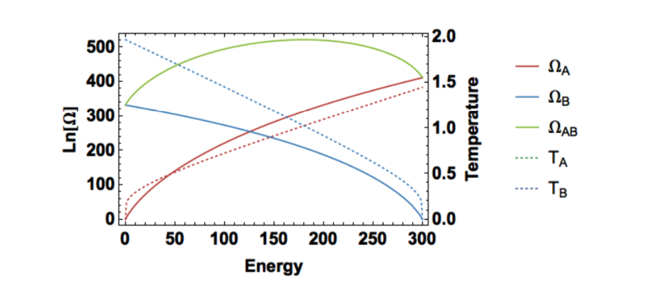 Figure 2: Multiplicity and temperature for each energy configuration when \(𝑁_A = 300, 𝑁_B = 200,\) and \(𝑞_T = 300\). Note that the temperatures are equal at maximum total multiplicity.
Results & Conclusions
Visual and tabular results summarize the results of simulations with different input values. Figure 3 shows the relative frequency of the possible energy macrostates for \(N_A=30\), \(N_B=70\), and \(q_T=40\). Table 2 shows that after 150,000 iterations our simulated averages and standard deviation are within 0.2% of the exact values. These values converge quickly for smaller systems, but a system this large has tremendous multiplicity (\(>10^{35}\)) so more iterations are necessary.
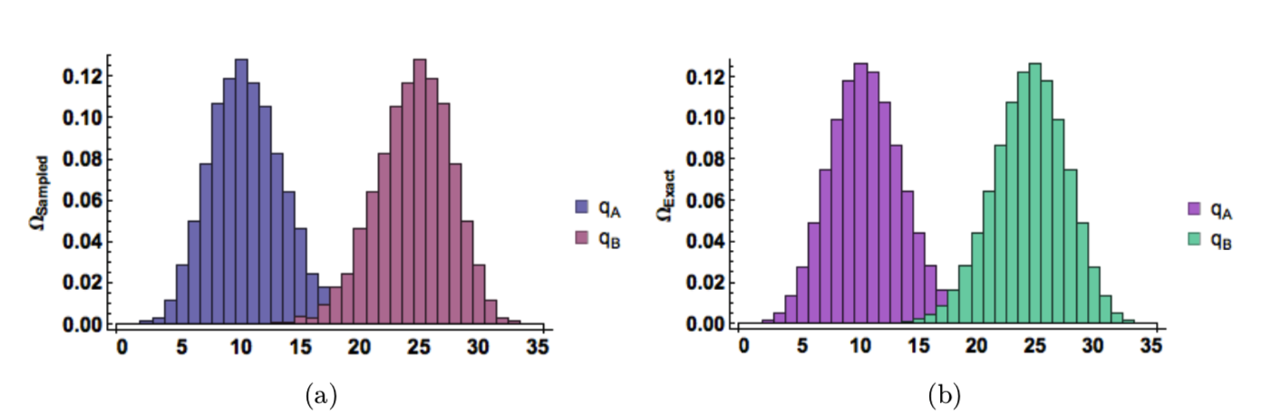 Figure 3: Normalized histograms given by (a) 150,000 random energy configurations (b) exact binomial distribution. (\(𝑁_A = 30, 𝑁_B = 70,\) and \(𝑞_T = 40\)).
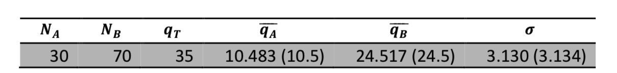 Table 2: Example results collected from 150,000 random energy distributions. The exact values are shown in parentheses for comparison.
As we expect from Equation (7) and the \(q/\sqrt{N}\) relationship for peak width, both total energy and system size affect the fluctuations in our simulations. Table 3 shows that the fluctuations increase when the total energy increases, and Table 4 shows that the fluctuations decrease when the number of oscillators increases. We also see that increasing the system size decreases accuracy since fewer of the possible microstates can be reached for such large system sizes.
With the exception of infinite conductivity, our system simulates a realistic scenario: an instrument measuring energy with many samples at a time. Such an instrument would effectively take an average of these samples and output the macroscopic measurement. Our simulated results and analytical results reveal that this measurement would fluctuate around the system’s most probable macrostate, which is determined by the multiplicity of the system’s microstates.
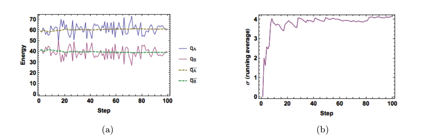 Figure 4: (a) Energy and average energy as a function of sample size. (b) Average standard deviation as a function of sample size. (\(N_A = 40, N_B = 60, q_T = 100\)).
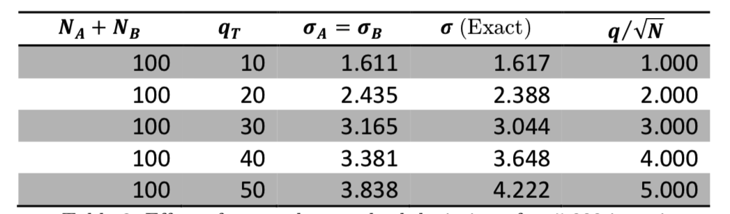 Table 3: Effect of \(q_T\) on the standard deviation after 5,000 iterations.
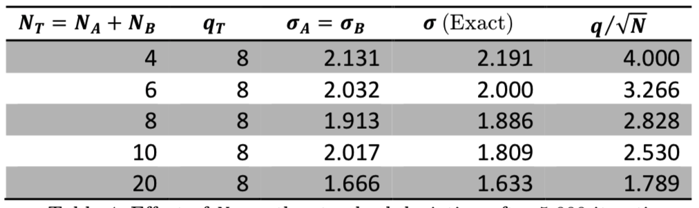 Table 4: Effect of \(N_T\) on the standard deviation after 5,000 iterations.
Energy Transport (Problems 2 & 3)
Mechanism of energy flow
To make our simulation more realistic, we now restrict energy transport so that our system no longer has infinite conductivity across the interface. In one dimension, Fourier’s law states that the heat flow in the x-direction is \[\begin{equation} q(x)=-K\frac{dT}{dx} \end{equation}\]
where \(T\) is the temperature and \(K\) is the thermal conductivity of the material. As we understood the problem, the program should use Fourier’s law in its simulation of energy transport. To do this, we created a quasi-classical model inspired by Fourier’s law, but analogous to the statistical mechanical model for Einstein solids. We isolated two characteristics of Fourier’s law that we strive to maintain:
 a)	The temperature difference determines the net energy flow.
 b)	𝐾 controls the rate of energy exchange.
We first calculate the amount of quanta to be exchanged in a given step using \[\begin{equation} \Delta Q = Max(1,K|T_B-T_A|) \end{equation}\]
Next we extract \(\Delta Q\) from randomly selected oscillators in the entire system. This \(\Delta Q\) is then randomly redistributed within then entire two-solid system. This process allows for transfer of energy both down and up the temperature gradient; however, it is statistically more likely for the redistribution of energy to occur down the gradient. Energy will flow in both directions, but the net flow is in the direction of thermal equilibrium, and the model converges to the most probable state.
Effect of system size, \(q_T\), and transport parameter
Figure 5 and Figure 6 show the energy in each solid as a function of time when system sizes and energy amounts are varied. As given by Equation (6), the ratio of oscillators of the solids still determines the equilibrium energies. Figure 5 shows that smaller systems reach equilibrium quicker but have greater fluctuations in energy. Figure 6 shows that a system with greater total energy has a more stable equilibrium (less fluctuations), but it reaches equilibrium more slowly.
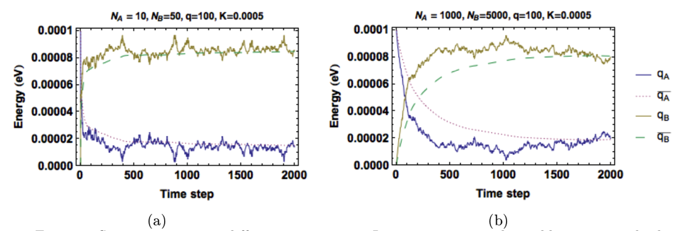 Figure 5: System response to different system sizes. Larger systems reach equilibrium more slowly, but have smaller fluctuations. (a) \(N_A=10, N_B=50\) (b)\(N_A=100,N_B=500\).
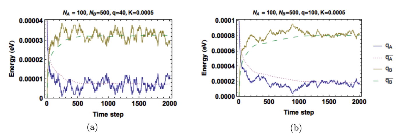 Figure 6: System response to different amounts of total energy. More energy increases time required to reach equilibrium, but also decreases the fluctuations. (a) \(q_T=40\)(b) \(q_T=100\).
Entropy and temperature in energy transport
When calculating the system’s thermodynamic properties, entropy and temperature, individual microstates are irrelevant. This is because the oscillator model has \(E_n=(n+\frac{1}{2})\hbar \omega\) and therefore \(E_{n+1}-E_n=\hbar \omega\). Each oscillator has equally spaced energy levels and the distribution of energy within each solid has no effect. Only the macroscopic properties, \(q_A\) and \(q_B\), matter. The entropy, 𝑆, was calculated using \[\begin{align} S_A(q_A,N_A) &=k_Bln(\Omega_A) \\[2em] S_B(q_B,N_B) &=k_Bln(\Omega_B) \\[2em] S_T(q_A,q_B,N_A,N_B) &=k_Bln(\Omega_{AB}) \\ \end{align}\]
where \(k_B\) is Boltzmann’s constant and \(\Omega_{AB}\) is given by Equation (3). Temperature was calculated using \[\begin{equation} T=(\frac{\partial S}{\partial E})^{-1}= [ \lim_{\Delta q \to0} \frac{S(q+\Delta q)-S(q-\Delta q)}{\Delta q}]^{-1}\cong\frac{2}{S(q+1)-S(q-1)} \end{equation}\]
Figure 7 shows plots of the entropy and temperature in each solid as time advances. As the system approaches equilibrium, the entropy of one solid decreases while the other increases, but the total entropy 𝑆! always increases. Once thermal equilibrium is reached, both solids fluctuate about the same average temperature. Looking at Figure 8, we see that our conductivity constant controls the equilibration rate. Comparing Figure 8a and Figure 8b shows that increasing \(K\) decreases the relaxation time but increases fluctuations in temperature and energy. To keep our values of temperature reasonable, we gave each unit of energy a value of \(1\times 10^{}-6eV\). This gave values of temperature around \(1000K\).
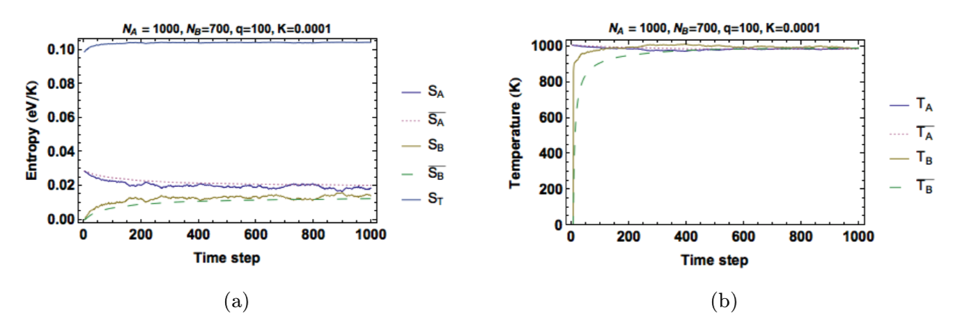 Figure 7: (a) Entropy and (b) temperature in each solid as a function of time. Configured with \(q_A(t_0)=100\) and \(q_B(t_0)=0\).
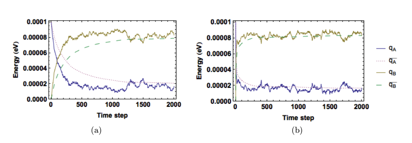 Figure 8: Faster convergence for higher conductivity. Both systems configured with \(q_A(t_0)=100, q_B(t_0)=0, N_A=1000\), and \(N_B=500\). Conductiity values were (a) \(K=1\times 10^{-4}\) (b) \(K=\times10^{-2}\).
Additional Thoughts
Metropolis Algorithm
We also ran a Metropolis algorithm to model energy transport. We created a random walker that randomly chooses any two adjacent grid points. This choice provides a candidate donor and recipient oscillator for energy exchange and corresponds to a new macrostate with multiplicity Ω!. We then compare Ω! to the multiplicity of the current state, Ω. When Ω! > Ω, the exchange is always accepted. When Ω! < Ω, the energy exchange is accepted if 𝑅𝑎𝑛𝑑𝑜𝑚 0,1 > Ω!/Ω.
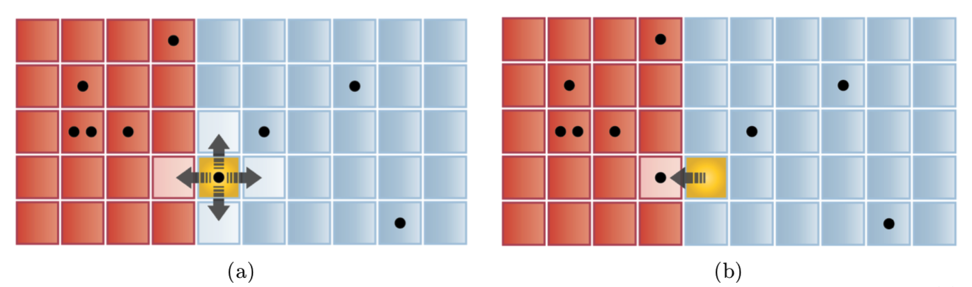 Figure 9: Illustration of a grid used in the Metropolis algorithm with \(N_A=20,N_B=30,H=5\). (a) A donor site has been chosen (yellow). (b) A recipient site has been chosen from the four adjacent sites and the candidate energy exchange will occur if \(𝑅𝑎𝑛𝑑𝑜𝑚 0,1 > \Omega^,/\Omega\).
A sample result is shown in Figure 10. The simulation behaves similarly to our Fourier model. Again, the energy values converge to those given in Equation (6), but the fluctuations in energy are smaller in this system and it converges to a very stable equilibrium. This is because the metropolis algorithm uses the degeneracy of the system itself to drive the simulation towards equilibrium.
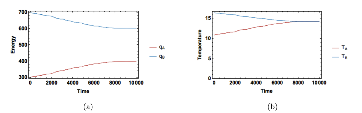 Figure 10: Results of metropolis algorithm with \(N_A=30,N_B=45,q_A(t_0)=700\), and \(q_B(t_0)=300\). Energy is shown in (a) and temperature in (b).
Simpler model for energy transport
As discussed in class, there is a simpler approach to energy transport that reproduces Fourier’s law indirectly rather than including the law explicitly. To compare this method with our previous results, we also implemented an approach along these lines. Each iteration consisted of two simple steps:
Step 1: Randomly distribute energy within each solid.
Step 2: Randomly distribute energy across the interface.
There are fewer interface sites than internal sites, so energy transport across the boundary is slower than within each solid. However, we also added a conductivity constant to further restrict the exchange rate. When the ratio of interface sites was equal to the ratio of oscillators, the results were very similar to our direct inclusion of Fourier’s law. An example is shown in Figure 11.
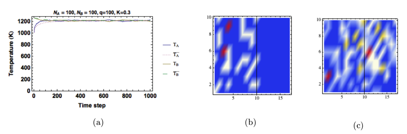 Figure 11: Results from the simpler model. (a) Temperature as a function of time step. (b) The distribution of energy in the solid at \(t=0\). (b) The distribution of energy in the solid at \(t=1000\).